pynibs package¶

Subpackages¶

Submodules¶

pynibs.coil module¶

All functions to operate on TMS coils go here, for example to create .xdmf files to visualize coil positions.

pynibs.coil.calc_coil_position_pdf(fn_rescon=None, fn_simpos=None, fn_exp=None, orientation='quaternions', folder_pdfplots=None)¶

Determines the probability density functions of the transformed coil position (x’, y’, z’) and quaternions of the coil orientations (x’’, y’’, z’’)

Parameters:

fn_rescon (str) – Filename of the results file from TMS experiments (results_conditions.csv)
fn_simpos (str) – Filename of the positions and orientation from TMS experiments (simPos.csv)
fn_exp (str) – Filename of experimental.csv file from experiments
orientation (str) – Type of orientation estimation: ‘quaternions’ or ‘euler’
folder_pdfplots (str) – Folder, where the plots of the fitted pdfs are saved (omitted if not provided)

Returns:

pdf_paras_location (list of list of np.ndarray) –

[n_conditions] Pdf parameters (limits and shape) of the coil position for x’, y’, and z’ for each:
- beta_paras … [p, q, a, b] (2 shape parameters and limits)
- moments … [data_mean, data_std, beta_mean, beta_std]
- p_value … p-value of the Kolmogorov Smirnov test
- uni_paras … [a, b] (limits)
pdf_paras_orientation_euler (list of np.ndarray) –

[n_conditions] Pdf parameters (limits and shape) of the coil orientation Psi, Theta, and Phi for each:
- beta_paras … [p, q, a, b] (2 shape parameters and limits)
- moments … [data_mean, data_std, beta_mean, beta_std]
- p_value … p-value of the Kolmogorov Smirnov test
- uni_paras … [a, b] (limits)
OP_mean (List of [3 x 4] np.ndarray) – [n_conditions] List of mean coil position and orientation for different conditions (global coordinate system)

$\begin{bmatrix} | & | & | & | \\ ori_x & ori_y & ori_z & pos \\ | & | & | & | \\ \end{bmatrix}$
OP_zeromean (list of [3 x 4 x n_con_each] np.ndarray [n_conditions]) – List over conditions containing zero-mean coil orientations and positions
V (list of [3 x 3] np.ndarrays [n_conditions]) – Transformation matrix of coil positions from global coordinate system to transformed coordinate system
P_transform (list of np.ndarray [n_conditions]) – List over conditions containing transformed coil positions [x’, y’, z’] of all stimulations (zero-mean, rotated by SVD)
quaternions (list of np.ndarray [n_conditions]) – List over conditions containing imaginary part of quaternions [x’’, y’’, z’’] of all stimulations

pynibs.coil.calc_coil_transformation_matrix(LOC_mean, ORI_mean, LOC_var, ORI_var, V)¶

Calculate the modified coil transformation matrix needed for SimNIBS based on location and orientation variations observed in the framework of uncertainty analysis

Parameters:

LOC_mean (np.ndarray of float) – (3), Mean location of TMS coil
ORI_mean (np.ndarray of float) –
(3 x 3) Mean orientations of TMS coil

$\begin{bmatrix} | & | & | \\ x & y & z \\ | & | & | \\ \end{bmatrix}$
LOC_var (np.ndarray of float) –
1. Location variation in normalized space (dx’, dy’, dz’), i.e. zero mean and projected on principal axes
ORI_var (np.ndarray of float) –
1. Orientation variation expressed in Euler angles [alpha, beta, gamma] in deg
V (np.ndarray of float) – (3x3) V-matrix containing the eigenvectors from _,_,V = numpy.linalg.svd

Returns:

mat (np.ndarray of float)
(4, 4) Transformation matrix containing 3 axis and 1 location vector –

$\begin{bmatrix} | & | & | & | \\ x & y & z & pos \\ | & | & | & | \\ 0 & 0 & 0 & 1 \\ \end{bmatrix}$

pynibs.coil.check_coil_position(points, hull)¶

Check if magnetic dipoles are lying inside head region

Parameters:

points (np.ndarray of float) – (N_points, 3) Coordinates (x,y,z) of magnetic dipoles
hull (Delaunay object or np.ndarray of float) – (N_surface_points, 3) Head surface data

Returns:

valid – Validity of coil position: TRUE: valid FALSE: unvalid

Return type:

bool

pynibs.coil.create_stimsite_from_exp_hdf5(fn_exp, fn_hdf, datanames=None, data=None, overwrite=False)¶

This takes an experiment.hdf5 file and creates an .hdf5 + .xdmf tuple for all coil positions for visualization.

Parameters:

fn_exp (str) – Path to experiment.hdf5
fn_hdf (str) – Filename for the resulting .hdf5 file. The .xdmf is saved with the same basename. Folder should already exist.
datanames (str or list of str, optional) – Dataset names for data
data (np.ndarray, optional) – Dataset array with shape = (len(poslist.pos), len(datanames()).
overwrite (bool, default: False) – Overwrite existing files.

pynibs.coil.create_stimsite_from_list(fn_hdf, poslist, datanames=None, data=None, overwrite=False)¶

This takes a list of matsimnibs-style coil position and orientations and creates an .hdf5 + .xdmf tuple for all positions.

Centers and coil orientations are written to disk, with optional data for each coil configuration.

Parameters:

fn_hdf (str) – Filename for the .hdf5 file. The .xdmf is saved with the same basename. Folder should already exist.
poslist (list of np.ndarray) – (4,4) Positions.
datanames (str or list of str, optional) – Dataset names for data.
data (np.ndarray, optional) – Dataset array with shape = (len(poslist.pos), len(datanames()).
overwrite (bool, defaul: False) – Overwrite existing files.

pynibs.coil.create_stimsite_from_matsimnibs(fn_hdf, matsimnibs, datanames=None, data=None, overwrite=False)¶

This takes a matsimnibs array and creates an .hdf5 + .xdmf tuple for all coil positions for visualization.

Centers and coil orientations are written disk.

Parameters:

fn_hdf (str) – Filename for the .hdf5 file. The .xdmf is saved with the same basename. Folder should already exist.
matsimnibs (np.ndarray) –
(4, 4, n_pos) Matsimnibs matrices containing the coil orientation (x,y,z) and position (p)

$\begin{bmatrix} | & | & | & | \\ x & y & z & p \\ | & | & | & | \\ 0 & 0 & 0 & 1 \\ \end{bmatrix}$
datanames (str or list of str, optional) – Dataset names for data.
data (np.ndarray, optional) – (len(poslist.pos), len(datanames).
overwrite (bool, default: False) – Overwrite existing files.

pynibs.coil.create_stimsite_from_tmslist(fn_hdf, poslist, datanames=None, data=None, overwrite=False)¶

This takes a :py:class:simnibs.sim_struct.TMSLIST from simnibs and creates an .hdf5 + .xdmf tuple for all positions.

Centers and coil orientations are written to disk, with optional data for each coil configuration.

Parameters:

fn_hdf (str) – Filename for the .hdf5 file. The .xdmf is saved with the same basename. Folder should already exist.
poslist (simnibs.sim_struct.TMSLIST) – poslist.pos[*].matsimnibs have to be set.
datanames (str or list of str, optional) – Dataset names for data.
data (np.ndarray, optional) – Dataset array with shape = (len(poslist.pos), len(datanames()).
overwrite (bool, default: False) – Overwrite existing files

pynibs.coil.create_stimsite_hdf5(fn_exp, fn_hdf, conditions_selected=None, sep='_', merge_sites=False, fix_angles=False, data_dict=None, conditions_ignored=None)¶

Reads results_conditions and creates an hdf5/xdmf pair with condition-wise centers of stimulation sites and coil directions as data.

Parameters:

fn_exp (str) – Path to results.csv.
fn_hdf (str) – Path where to write file. Gets overridden if already existing.
conditions_selected (str or list of str, optional) – List of conditions returned by the function, the others are omitted. If None, all conditions are returned.
sep (str, default: "_") – Separator between condition label and angle (e.g. M1_0, or M1-0).
merge_sites (bool) – If true, only one coil center per site is generated.
fix_angles (bool) – rename 22.5 -> 0, 0 -> -45, 67.5 -> 90, 90 -> 135.
data_dict (dict ofnp.ndarray of float [n_stimsites] (optional), default: None) – Dictionary containing data corresponding to the stimulation sites (keys).
conditions_ignored (str or list of str, optional) – Conditions, which are not going to be included in the plot.

Returns:

<Files> – Contains information about condition-wise stimulation sites and coil directions (fn_hdf)

Return type:

hdf5/xdmf file pair

Example

pynibs.create_stimsite_hdf5('/exp/1/experiment_corrected.csv',
                            '/stimsite', True, True)

pynibs.coil.get_coil_dipole_pos(coil_fn, matsimnibs)¶

Apply transformation to coil dipoles and return position.

Parameters:

coil_fn (str) – Filename of coil .ccd file.
matsimnibs (np.ndarray of float) – Transformation matrix.

Returns:

dipoles_pos – (N, 3) Cartesian coordinates (x, y, z) of coil magnetic dipoles.

Return type:

np.ndarray

pynibs.coil.get_invalid_coil_parameters(param_dict, coil_position_mean, svd_v, del_obj, fn_coil, fn_hdf5_coilpos=None)¶

Finds gpc parameter combinations, which place coil dipoles inside subjects head. Only endpoints (and midpoints) of the parameter ranges are examined.

get_invalid_coil_parameters(param_dict, pos_mean, v, del_obj, fn_coil, fn_hdf5_coilpos=None)

Parameters:

param_dict (dict) – Dictionary containing dictionary with 'limits' and 'pdfshape'. keys: 'x', 'y', 'z', 'psi', 'theta', 'phi'.
coil_position_mean (np.ndarray) – (3, 4) Mean coil positions and orientations.
svd_v (np.ndarray) – (3, 3) SVD matrix V.
del_obj (scipy.spatial.Delaunay) – Skin surface.
fn_coil (str) – Filename of coil .ccd file.
fn_hdf5_coilpos (str) – Filename of .hdf5 file to save coil_pos in (incl. path and .hdf5 extension).

Returns:

fail_params – Index and combination of failed parameter.

Return type:

list of int

pynibs.coil.random_walk_coil(start_mat, n_steps, fn_mesh_hdf5, angles_dev=3, distance_low=1, distance_high=4, angles_metric='deg', coil_pos_fn=None)¶

Computes random walk coil positions/orientations for a SimNIBS matsimnibs coil pos/ori.

Parameters:

start_mat (np.ndarry) – (4, 4) SimNIBS matsimnibs.
n_steps (int) – Number of steps to walk.
fn_mesh_hdf5 (str) – .hdf5 mesh filename, used to compute skin-coil distances.
angles_dev (float or list of float, default: 3) – Angles deviation,`` np.random.normal(scale=angles_dev)``. If list, angles_dev = [alpha, beta, theta].
distance_low (float, default: 1) – Minimum skin-coil distance.
distance_high (float, default: 4) – Maximum skin-coil distance.
angles_metric (str, default: 'deg') – One of ('deg', 'rad').
coil_pos_fn (str, optional) – If provided, .hdf5/.xdmf tuple is written with coil positions/orientations.

Returns:

walked_coils (np.ndarray) – (4, 4, n_steps + 1) coil positions / orientations.
<file> (.hdf5/.xdmf file tupel with n_steps + 1 coil positions/orientations.)

pynibs.coil.sort_opt_coil_positions(fn_coil_pos_opt, fn_coil_pos, fn_out_hdf5=None, root_path='/0/0/', verbose=False, print_output=False)¶

Sorts coil positions according to Traveling Salesman problem

Parameters:

fn_coil_pos_opt (str) – Name of .hdf5 file containing the optimal coil position indices
fn_coil_pos (str) – Name of .hdf5 file containing the matsimnibs matrices of all coil positions
fn_out_hdf5 (str) – Name of output .hdf5 file (will be saved in the same format as fn_coil_pos_opt)
verbose (bool, default: False) – Print output messages
print_output (bool or str, default: False) – Print output image as .png file showing optimal path

Return type:

<file> .hdf5 file containing the sorted optimal coil position indices

pynibs.coil.test_coil_position_gpc(parameters)¶: Testing valid coil positions for gPC analysis

pynibs.coil.write_coil_pos_hdf5(fn_hdf, centers, m0, m1, m2, datanames=None, data=None, overwrite=False)¶

Creates a .hdf5 + .xdmf file tuple for all coil positions. Coil centers and coil orientations are saved, and - optionally - data for each position if data and datanames are provided.

Parameters:

fn_hdf (str) – Filename for the .hdf5 file. The .xdmf is saved with the same basename. Folder should already exist.
centers (np.ndarray of float) – (n_pos, 3) Coil positions.
m0 (np.ndarray of float) – (n_pos, 3) Coil orientation x-axis (looking at the active (patient) side of the coil pointing to the right).
m1 (np.ndarray of float) – (n_pos, 3) Coil orientation y-axis (looking at the active side of the coil pointing up away from the handle).
m2 (np.ndarray of float) – (n_pos, 3) Coil orientation z-axis (looking at the active (patient) side of the coil pointing to the patient).
datanames (str or list of str, optional) – (n_data) Dataset names for data
data (np.ndarray, optional) – (n_pos, n_data) Dataset array with (len(poslist.pos), len(datanames()).
overwrite (bool, default: False) – Overwrite existing files.

pynibs.freesurfer module¶

This holds methods to interact with FreeSurfer ([1]), for example to translate FreeSurfer files into Paraview readable .vtk files.

References

[1]

Dale, A.M., Fischl, B., Sereno, M.I., 1999. Cortical surface-based analysis. I. Segmentation and surface reconstruction. Neuroimage 9, 179-194.

pynibs.freesurfer.data_sub2avg(fn_subject_obj, fn_average_obj, hemisphere, fn_in_hdf5_data, data_hdf5_path, data_label, fn_out_hdf5_geo, fn_out_hdf5_data, mesh_idx=0, roi_idx=0, subject_data_in_center=True, data_substitute=-1, verbose=True, replace=True, reg_fn='sphere.reg')¶

Maps the data from the subject space to the average template. If the data is given only in an ROI, the data is mapped to the whole brain surface.

Parameters:

fn_subject_obj (str) – Filename of subject object .hdf5 file (incl. path), e.g. .../probands/subjectID/subjectID.hdf5
fn_average_obj (str) – Filename of average template object .pkl file (incl. path), e.g. .../probands/avg_template/avg_template.hdf5.
hemisphere (str) – Define hemisphere to work on ('lh' or 'rh' for left or right hemisphere, respectively).
fn_in_hdf5_data (str) – Filename of .hdf5 data input file containing the subject data.
data_hdf5_path (str) – Path in .hdf5 data file where data is stored (e.g. '/data/tris/').
data_label (str or list of str) – Label of datasets contained in hdf5 input file to map.
fn_out_hdf5_geo (str) – Filename of .hdf5 geo output file containing the geometry information.
fn_out_hdf5_data (str) – Filename of .hdf5 data output file containing the mapped data.
mesh_idx (int) – Index of mesh used in the simulations.
roi_idx (int) – Index of region of interest used in the simulations.
subject_data_in_center (bool, default: True) – Specify if the data is given in the center of the triangles or in the nodes.
data_substitute (float) – Data substitute with this number for all points outside the ROI mask
verbose (bool) – Verbose output (Default: True)
replace (bool) – Replace output files (Default: True)
reg_fn (str) – Sphere.reg fn

Returns:

<Files> – Geometry and corresponding data files to plot with Paraview:

fn_out_hdf5_geo.hdf5: geometry file containing the geometry information of the average template
fn_out_hdf5_data.hdf5: geometry file containing the data

Return type:

.hdf5 files

pynibs.freesurfer.freesurfer2vtk(in_fns, out_folder, hem='lh', surf='pial', prefix=None, fs_subject='fsaverage', fs_subjects_dir=None)¶

Transform multiple FreeSurfer .mgh files into one .vtk file. This can be read with Paraview and others.

Parameters:

in_fns (list of str or str) – Input filenames.
out_folder (str) – Output folder.
hem (str, default: 'lh') – Which hemisphere: 'lh' or 'rh'.
surf (str, default: 'pial') – Which FreeSurfer surface: 'pial', 'inflated', …
prefix (str, optional) – Prefix to add to each filename.
fs_subject (str, default: 'fsaverage') – FreeSurfer subject.
fs_subjects_dir (str, optional) – FreeSurfer subjects directory. If not provided, read from environment.

Returns:

<File> – One .vtk file with data as overlays from all .mgh files provided

Return type:

out_folder/{prefix}_{hem}_{surf}.vtk

pynibs.freesurfer.make_average_subject(subjects, subject_dir, average_dir, fn_reg='sphere.reg')¶

Generates the average template from a list of subjects using the FreeSurfer average.

Parameters:

subjects (list of str) – Paths of subjects directories, where the FreeSurfer files are located, e.g. for simnibs mri2mesh .../fs_SUBJECT_ID.
subject_dir (str) – Temporary subject directory of FreeSurfer (symlinks of subjects will be generated in there and average template will be temporarily stored before it is copied to average_dir).
average_dir (str) – path to directory where average template will be stored, e.g. probands/avg_template_15/mesh/0/fs_avg_template_15.
fn_reg (str, default: 'sphere.reg' --> ?h.sphere.reg>) – Filename suffix of FreeSurfer registration file containing registration information to template.

Returns:

<Files> – Average template in average_dir and registered curvature files, ?h.sphere.reg in subjects/surf folders.

Return type:

.tif and .reg files

pynibs.freesurfer.make_group_average(subjects=None, subject_dir=None, average=None, hemi='lh', template='mytemplate', steps=3, n_cpu=2, average_dir=None)¶

Creates a group average from scratch, based on one subject. This prevents for example the fsaverage problems of large elements at M1, etc. This is an implemntation of [2] ‘Creating a registration template from scratch (GW)’.

References

[2]

https://surfer.nmr.mgh.harvard.edu/fswiki/SurfaceRegAndTemplates

Parameters:

subjects (list of str) – List of FreeSurfer subjects names.
subject_dir (str) – Temporary subject directory of FreeSurfer (symlinks of subjects will be generated in there and average template will be temporarily stored before it is copied to average_dir).
average (str, default: subjects[0]) – Which subject to base new average template on.
hemi (str, default: 'lh') –
Which hemisphere: lh or rh.

Deprecated since version 0.0.1: Don’t use any more.
template (str, default: 'mytemplate') – Basename of new template.
steps (int, default: 2) – Number of iterations.
n_cpu (int, default: 4) – How many cores for multithreading.
average_dir (str) – Path to directory where average template will be stored, e.g. probands/avg_template_15/mesh/0/fs_avg_template_15.

Returns:

<File> (.tif file) – SUBJECT_DIR/TEMPLATE*.tif, TEMPLATE0.tif based on AVERAGE, rest on all subjects.
<File> (.myreg file) – SUBJECT_DIR/SUBJECT*/surf/HEMI.sphere.myreg*.
<File> (.tif file) – Subject wise sphere registration based on TEMPLATE*.tif.

pynibs.freesurfer.read_curv_data(fname_curv, fname_inf, raw=False)¶

Read curvature data provided by FreeSurfer with optional normalization.

Parameters:

fname_curv (str) – Filename of the FreeSurfer curvature file (e.g. ?h.curv), contains curvature data in nodes can be found in mri2mesh proband folder: proband_ID/fs_ID/surf/?h.curv.
fname_inf (str) – Filename of inflated brain surface (e.g. ?h.inflated), contains points and connectivity data of surface can be found in mri2mesh proband folder: proband_ID/fs_ID/surf/?h.inflated.
raw (bool) – If raw-data is returned or if the data is normalized to -1 for neg. and +1 for pos. curvature.

Returns:

curv – Curvature data in element centers.

Return type:

np.ndarray of float or int

pynibs.hdf5_io module¶

pynibs.hdf5_io.create_fibre_geo_hdf5(fn_fibres_hdf5, overwrite=True)¶

Reformats geometrical fibre data and adds a /plot subfolder containing geometrical fibre data including connectivity

Parameters:

fn_fibres_hdf5 (str) – Path to fibre.hdf5 file containing the original fibre data
overwrite (bool) – Overwrites existing /plot subfolder in .hdf5 file

pynibs.hdf5_io.create_fibre_xdmf(fn_fibre_geo_hdf5, fn_fibre_data_hdf5=None, overwrite=True, fibre_points_path='fibre_points', fibre_con_path='fibre_con', fibre_data_path='')¶

Creates .xdmf file to plot fibres in Paraview

Parameters:

fn_fibre_geo_hdf5 (str) – Path to fibre_geo.hdf5 file containing the geometry (in /plot subfolder created with create_fibre_geo_hdf5())
fn_fibre_data_hdf5 (str (optional) default: None) – Path to fibre_data.hdf5 file containing the data to plot (in parent folder)
fibre_points_path (str (optional) default: fibre_points) – Path to fibre point array in .hdf5 file
fibre_con_path (str (optional) default: fibre_con) – Path to fibre connectivity array in .hdf5 file
fibre_data_path (str (optional) default: "") – Path to parent data folder in data.hdf5 file (Default: no parent folder)

Returns:

<File>

Return type:

.xdmf file for Paraview

pynibs.hdf5_io.create_position_path_xdmf(sorted_fn, coil_pos_fn, output_xdmf, stim_intens=None, coil_sorted='/0/0/coil_seq')¶

Creates one .xdmf file that allows paraview plottings of coil position paths.

A set of coil positions plotted to show the path of coil movement.

Paraview can be used to visualize the order of realized stimulation positions.

Parameters:

sorted_fn (str) – .hdf5 filename with position indices, values, intensities from pynibs.sort_opt_coil_positions().
coil_pos_fn (str) – .hdf5 filename with original set of coil positions. Indices from sorted_fn are mapped to this. Either ‘/matsimnibs’ or ‘m1’ and ‘m2’ datasets.
output_xdmf (str) –
stim_intens (int, optional) – Intensities are multiplied by this factor.
coil_sorted (str) – Path to coil positions in sorted_fn

Returns:

output_xdmf

Return type:

<file>

pynibs.hdf5_io.data_superimpose(fn_in_hdf5_data, fn_in_geo_hdf5, fn_out_hdf5_data, data_hdf5_path='/data/tris/', data_substitute=-1, normalize=False)¶

Overlaying data stored in .hdf5 files except in regions where data_substitute is found. These points are omitted in the analysis and will be replaced by data_substitute instead.

Parameters:

fn_in_hdf5_data (list of str) – Filenames of .hdf5 data files with common geometry, e.g. generated by pynibs.data_sub2avg(…).
fn_in_geo_hdf5 (str) – Geometry .hdf5 file, which corresponds to the .hdf5 data files.
fn_out_hdf5_data (str) – Filename of .hdf5 data output file containing the superimposed data.
data_hdf5_path (str) – Path in .hdf5 data file where data is stored (e.g. '/data/tris/').
data_substitute (float or np.NaN, default: -1) – Data substitute with this number for all points in the inflated brain, which do not belong to the given data set.
normalize (bool or str, default: False) –
Decide if individual datasets are normalized w.r.t. their maximum values before they are superimposed.
- ’global’: global normalization w.r.t. maximum value over all datasets and subjects
- ’dataset’: dataset wise normalization w.r.t. maximum of each dataset individually (over subjects)
- ’subject’: subject wise normalization (over datasets)

Returns:

<File> – Overlayed data.

Return type:

.hdf5 file

pynibs.hdf5_io.hdf_2_ascii(hdf5_fn)¶

Prints out structure of given .hdf5 file.

Parameters:: hdf5_fn (str) – Filename of .hdf5 file.
Returns:: h5 – Structure of .hdf5 file
Return type:: items

pynibs.hdf5_io.load_mesh_hdf5(fname)¶

Loading mesh from .hdf5 file and setting up TetrahedraLinear class.

Parameters:: fname (str) – Name of .hdf5 file (incl. path)
Returns:: obj – TetrahedraLinear object
Return type:: pynibs.mesh.mesh_struct.TetrahedraLinear

Example

.hdf5 file format and contained groups. The content of .hdf5 files can be shown using the tool HDFView (https://support.hdfgroup.org/products/java/hdfview/)

mesh
I---/elm
I    I--/elm_number          [1,2,3,...,N_ele]           Running index over all elements starting at 1,
                                                            triangles and tetrahedra
I    I--/elm_type            [2,2,2,...,4,4]             Element type: 2 triangles, 4 tetrahedra
I    I--/node_number_list    [1,5,6,0;... ;1,4,8,9]      Connectivity of triangles [X, X, X, 0] and tetrahedra
                                                                    [X, X, X, X]
I    I--/tag1                [1001,1001, ..., 4,4,4]     Surface (100X) and domain (X) indices with 1000 offset
                                                                     for surfaces
I    I--/tag2                [   1,   1, ..., 4,4,4]     Surface (X) and domain (X) indices w/o offset
I
I---/nodes
I    I--/node_coord          [1.254, 1.762, 1.875;...]   Node coordinates in (mm)
I    I--/node_number         [1,2,3,...,N_nodes]         Running index over all points starting at 1
I    I--/units               ["mm"]                      .value is unit of geometry
I
I---/fields
I    I--/E/value             [E_x_1, E_y_1, E_z_1;...]   Electric field in all elms, triangles and tetrahedra
I    I--/J/value             [J_x_1, J_y_1, J_z_1;...]   Current density in all elms, triangles and tetrahedra
I    I--/normE/value         [normE_1,..., normE_N_ele]  Magnitude of electric field in all elements,
                                                                    triangles and tetrahedra
I    I--/normJ/value         [normJ_1,..., normJ_N_ele]  Magnitude of current density in all elements,
                                                                    triangles and tetrahedra

/data
I---/potential               [phi_1, ..., phi_N_nodes]   Scalar electric potential in nodes (size N_nodes)
I---/dAdt                    [A_x_1, A_y_1, A_z_1,...]   Magnetic vector potential (size 3xN_nodes)

pynibs.hdf5_io.load_mesh_msh(fname)¶

Loading mesh from .msh file and return TetrahedraLinear object.

Parameters:: fname (str) – .msh filename (incl. path)
Returns:: obj
Return type:: pynibs.mesh.mesh_struct.TetrahedraLinear

pynibs.hdf5_io.msh2hdf5(fn_msh=None, skip_roi=False, skip_layer=True, include_data=False, approach='mri2mesh', subject=None, mesh_idx=None)¶

Transforms mesh from .msh to .hdf5 format. Mesh is read from subject object or from fn_msh.

Parameters:

fn_msh (str, optional) – Filename of .msh file.
skip_roi (bool, default: False) – Skip generating ROI in .hdf5
skip_layer (book, default: True) – Don’t create gm layers.
include_data (bool, default: False) – Also convert data in .msh file to .hdf5 file
subject (pynibs.Subject, optional) – Subject information, ust be set to use skip_roi=False..
mesh_idx (int or list of int or str or list of str, optional) – Mesh index, the conversion from .msh to .hdf5 is conducted for.
approach (str) –
Approach the headmodel was created with (“mri2mesh” or “headreco”).

Deprecated since version 0.0.1: Not supported any more.

Returns:

<File> – .hdf5 file with mesh information

Return type:

.hdf5 file

pynibs.hdf5_io.print_attrs(name, obj)¶

Helper function for hdf_2_ascii(). To be called from h5py.Group.visititems()

Parameters:

name (str) – Name of structural element
obj (object) – Structural element

Returns:

<Print>

Return type:

Structure of .hdf5 file

pynibs.hdf5_io.read_arr_from_hdf5(fn_hdf5, folder)¶

Reads array from and .hdf5 files and returns as list: Strings are returned as np.bytes_ to str and ‘None’ to None

Parameters:

fn_hdf5 (str) – Filename of .hdf5 file
folder (str) – Folder inside .hdf5 file to read

Returns:

data_from_hdf5 – List containing data from .hdf5 file

Return type:

list

pynibs.hdf5_io.read_data_hdf5(fname)¶

Reads phi and dA/dt data from .hdf5 file (phi and dAdt are given in the nodes).

Parameters:

fname (str) – Filename of .hdf5 data file

Returns:

phi (np.ndarray of float [N_nodes]) – Electric potential in the nodes of the mesh
da_dt (np.ndarray of float [N_nodesx3]) – Magnetic vector potential in the nodes of the mesh

pynibs.hdf5_io.read_dict_from_hdf5(fn_hdf5, folder)¶

Read all arrays from from hdf5 file and return them as dict

Parameters:

fn_hdf5 (str) – Filename of .hdf5 file
folder (str) – Folder inside .hdf5 file to read

Returns:

d – Dictionary from .hdf5 file folder

Return type:

dict

pynibs.hdf5_io.simnibs_results_msh2hdf5(fn_msh, fn_hdf5, S, pos_tms_idx, pos_local_idx, subject, mesh_idx, mode_xdmf='r+', n_cpu=4, verbose=False, overwrite=False, mid2roi=False)¶

Converts simnibs .msh results file(s) to .hdf5 / .xdmf tuple.

Parameters:

fn_msh (str list of str) – Filenames (incl. path) of .msh results files from SimNIBS.
fn_hdf5 (str or list of str) – Filenames (incl. path) of .hdf5 results files.
S (Simnibs Session object) – Simnibs Session object the simulations are conducted with.
pos_tms_idx (list of int) – Index of the simulation w.r.t. to the simnibs TMSList (inside Session object S) For every coil a separate TMSList exists, which contains multiple coil positions.
pos_local_idx (list of int) – Index of the simulation w.r.t. to the simnibs POSlist in the TMSList (inside Session object S) For every coil a separate TMSList exists, which contains multiple coil positions.
subject (pynibs.subject.Subject) – Subject object.
mesh_idx (int or str) – Mesh id.
mode_xdmf (str, default: "r+") – Mode to open hdf5_geo file to write xdmf. If hdf5_geo is already separated in tets and tris etc., the file is not changed, use “r” to avoid IOErrors in case of parallel computing.
n_cpu (int) – Number of processes.
verbose (bool, default: False) – Print output messages.
overwrite (bool, default: False) – Overwrite .hdf5 file if existing.
mid2roi (bool or string, default: False) – If the mesh contains ROIs and the e-field was calculated in the midlayer using simnibs (S.map_to_surf = True), the midlayer results will be mapped from the simnibs midlayer to the ROIs (takes some time for large ROIs).

Returns:

<File> – .hdf5 file containing the results. An .xdmf file is also created to link the results with the mesh .hdf5 file of the subject

Return type:

.hdf5 file

pynibs.hdf5_io.simnibs_results_msh2hdf5_workhorse(fn_msh, fn_hdf5, S, pos_tms_idx, pos_local_idx, subject, mesh_idx, mode_xdmf='r+', verbose=False, overwrite=False, mid2roi=False)¶

Converts simnibs .msh results file to .hdf5 (including midlayer data if desired)

Parameters:

fn_msh (list of str) – Filenames (incl. path) of .msh results files from simnibs
fn_hdf5 (str or list of str) – Filenames (incl. path) of .hdf5 results files
S (Simnibs Session object) – Simnibs Session object the simulations are conducted with
pos_tms_idx (list of int) – Index of the simulation w.r.t. to the simnibs TMSList (inside Session object S) For every coil a separate TMSList exists, which contains multiple coil positions.
pos_local_idx (list of int) – Index of the simulation w.r.t. to the simnibs POSlist in the TMSList (inside Session object S) For every coil a separate TMSList exists, which contains multiple coil positions.
subject (Subject object) – Subject object loaded from .pkl file
mesh_idx (int) – Mesh index
mode_xdmf (str, default: "r+") – Mode to open hdf5_geo file to write xdmf. If hdf5_geo is already separated in tets and tris etc, the file is not changed, use “r” to avoid IOErrors in case of parallel computing.
verbose (bool, default: False) – Print output messages
overwrite (bool, default: False) – Overwrite .hdf5 file if existing
mid2roi (bool, list of string, or string, default:False) – If the mesh contains ROIs and the e-field was calculated in the midlayer using simnibs (S.map_to_surf = True), the midlayer results will be mapped from the simnibs midlayer to the ROIs (takes some time for large ROIs)

Returns:

<File> – .hdf5 file containing the results. An .xdmf file is also created to link the results with the mesh .hdf5 file of the subject

Return type:

.hdf5 file

pynibs.hdf5_io.split_hdf5(hdf5_in_fn, hdf5_geo_out_fn='', hdf5_data_out_fn=None)¶

Splits one hdf5 into one with spatial data and one with statistical data. If coil data is present in hdf5_in, it is saved in hdf5Data_out. If new spatial data is added to file (curve, inflated, whatever), add this to the geogroups variable.

Parameters:

hdf5_in_fn (str) – Filename of .hdf5 input file
hdf5_geo_out_fn (str) – Filename of .hdf5 .geo output file
hdf5_data_out_fn (str) – Filename of .hdf5 .data output file (ff none, remove data from hdf5_in)

Returns:

<File> (.hdf5 file) – hdf5Geo_out_fn (spatial data)
<File> (.hdf5 file) – hdf5Data_out_fn (data)

pynibs.hdf5_io.write_arr_to_hdf5(fn_hdf5, arr_name, data, overwrite_arr=True, verbose=False, check_file_exist=False)¶

Takes an array and adds it to an hdf5 file

If data is list of dict, write_dict_to_hdf5() is called for each dict with adapted hdf5-folder name Otherwise, data is casted to np.ndarray and dtype of unicode data casted to '|S'.

Parameters:

fn_hdf5 (str) – Filename of .hdf5 file
arr_name (str) – Complete path in .hdf5 file with array name
data (ndarray, list or dict) – Data to write
overwrite_arr (bool, default: True) – Overwrite existing array
verbose (bool, default: False) – Print information

pynibs.hdf5_io.write_coil_sequence_xdmf(coil_pos_fn, data, vec1, vec2, vec3, output_xdmf)¶

pynibs.hdf5_io.write_data_hdf5(out_fn, data, data_names, hdf5_path='/data', mode='a')¶

Creates a .hdf5 file with data.

Parameters:

out_fn (str) – Filename of output .hdf5 file containing the geometry information
data (np.ndarray or list of nparrays of float) – Data to save in hdf5 data file
data_names (str or list of str) – Labels of data
hdf5_path (str) – Folder in .hdf5 geometry file, where the data is saved in (Default: /data)
mode (str, default: "a") – Mode: “a” append, “w” write (overwrite)

Returns:

<File> – File containing the stored data

Return type:

.hdf5 file

Example

File structure of .hdf5 data file

data
|---/data_names[0]          [data[0]]           First dataset
|---/    ...                   ...                  ...
|---/data_names[N-1]        [data[N-1]]         Last dataset

pynibs.hdf5_io.write_data_hdf5_surf(data, data_names, data_hdf_fn_out, geo_hdf_fn, replace=False, replace_array_in_file=True)¶

Saves surface data to .hdf5 data file and generates corresponding .xdmf file linking both. The directory of data_hdf_fn_out and geo_hdf_fn should be the same, as only basenames of files are stored in the .xdmf file.

Parameters:

data (np.ndarray or list) – (N_points_ROI, N_components) Data to map on surfaces.
data_names (str or list) – Names for datasets.
data_hdf_fn_out (str) – Filename of .hdf5 data file.
geo_hdf_fn (str) – Filename of .hdf5 geo file containing the geometry information (has to exist).
replace (bool, default: False) – Replace existing .hdf5 and .xdmf file completely.
replace_array_in_file (bool, default: True) – Replace existing array in file.

Returns:

<File> (.hdf5 file) – data_hdf_fn_out.hdf5 containing data
<File> (.xdmf file) – data_hdf_fn_out.xdmf containing information about .hdf5 file structure for Paraview

Example

File structure of .hdf5 data file

/data
|---/tris
|      |---dataset_0    [dataset_0]    (size: N_dataset_0 x M_dataset_0)
|      |---   ...
|      |---dataset_K   [dataset_K]     (size: N_dataset_K x M_dataset_K)

pynibs.hdf5_io.write_data_hdf5_vol(data, data_names, data_hdf_fn_out, geo_hdf_fn, replace=False, replace_array_in_file=True)¶

Parameters:

data (np.ndarray or list) – (N_points_ROI, N_components) Data to map on surfaces.
data_names (str or list) – Names for datasets.
data_hdf_fn_out (str) – Filename of .hdf5 data file.
geo_hdf_fn (str) – Filename of .hdf5 geo file containing the geometry information (has to exist).
replace (bool, default: False) – Replace existing .hdf5 and .xdmf file completely.
replace_array_in_file (bool, default: True) – Replace existing array in file.

Returns:

<File> (.hdf5 file) – data_hdf_fn_out.hdf5 containing data
<File> (.xdmf file) – data_hdf_fn_out.xdmf containing information about .hdf5 file structure for Paraview

Example

File structure of .hdf5 data file

/data
|---/tris
|      |---dataset_0    [dataset_0]    (size: N_dataset_0 x M_dataset_0)
|      |---   ...
|      |---dataset_K   [dataset_K]     (size: N_dataset_K x M_dataset_K)

pynibs.hdf5_io.write_dict_to_hdf5(fn_hdf5, data, folder, check_file_exist=False, verbose=False)¶

Takes dict (from subject.py) and passes its keys to write_arr_to_hdf5()

fn_hdf5:folder/
              |--key1
              |--key2
              |...

Parameters:

fn_hdf5 (str) –
data (dict or pynibs.Mesh) –
folder (str) –
verbose (bool) –
check_file_exist (bool) –

pynibs.hdf5_io.write_geo_hdf5(out_fn, msh, roi_dict=None, hdf5_path='/mesh')¶

Creates a .hdf5 file with geometry data from mesh including region of interest(s).

Parameters:

out_fn (str) – Output hdf5 filename for mesh’ geometry information.
msh (pynibs.mesh.mesh_struct.TetrahedraLinear) – Mesh to write to file.
roi_dict (dict of (RegionOfInterestSurface or RegionOfInterestVolume)) – Region of interest (surface and/or volume) information.
hdf5_path (str, default: '/mesh') – Path in output file to store geometry information.

Returns:

<File> – File containing the geometry information

Return type:

.hdf5 file

Example

File structure of .hdf5 geometry file

mesh
I---/elm
I    I--/elm_number             [1,2,3,...,N_ele]        Running index over all elements starting at 1
                                                            (triangles and tetrahedra)
I    I--/elm_type               [2,2,2,...,4,4]          Element type: 2 triangles, 4 tetrahedra
I    I--/tag1                [1001,1001, ..., 4,4,4]     Surface (100X) and domain (X) indices with 1000
                                                                    offset for surfaces
I    I--/tag2                [   1,   1, ..., 4,4,4]     Surface (X) and domain (X) indices w/o offset
I    I--/triangle_number_list   [1,5,6;... ;1,4,8]       Connectivity of triangles [X, X, X]
I    I--/tri_tissue_type        [1,1, ..., 3,3,3]        Surface indices to differentiate between surfaces
I    I--/tetrahedra_number_list [1,5,6,7;... ;1,4,8,12]  Connectivity of tetrahedra [X, X, X, X]
I    I--/tet_tissue_type        [1,1, ..., 3,3,3]        Volume indices to differentiate between volumes
I    I--/node_number_list       [1,5,6,0;... ;1,4,8,9]   Connectivity of triangles [X, X, X, 0] and
                                                            tetrahedra [X, X, X, X]
I
I---/nodes
I    I--/node_coord          [1.254, 1.762, 1.875;...]   Node coordinates in (mm)
I    I--/node_number         [1,2,3,...,N_nodes]         Running index over all points starting at 1
I    I--/units               ['mm']                      .value is unit of geometry

roi_surface
I---/0                                                           Region of Interest number
I    I--/node_coord_up              [1.254, 1.762, 1.875;...]    Coordinates of upper surface points
I    I--/node_coord_mid             [1.254, 1.762, 1.875;...]    Coordinates of middle surface points
I    I--/node_coord_low             [1.254, 1.762, 1.875;...]    Coordinates of lower surface points
I    I--/tri_center_coord_up        [1.254, 1.762, 1.875;...]    Coordinates of upper triangle centers
I    I--/tri_center_coord_mid       [1.254, 1.762, 1.875;...]    Coordinates of middle triangle centers
I    I--/tri_center_coord_low       [1.254, 1.762, 1.875;...]    Coordinates of lower triangle centers
I    I--/node_number_list           [1,5,6,0;... ;1,4,8,9]       Connectivity of triangles [X, X, X]
I    I--/delta                      0.5                          Distance parameter between GM and WM surface
I    I--/tet_idx_tri_center_up      [183, 913, 56, ...]          Tetrahedra indices where triangle center of
                                                                    upper surface are lying in
I    I--/tet_idx_tri_center_mid     [185, 911, 58, ...]          Tetrahedra indices where triangle center of
                                                                    middle surface are lying in
I    I--/tet_idx_tri_center_low     [191, 912, 59, ...]          Tetrahedra indices where triangle center of
                                                                    lower surface are lying in
I    I--/tet_idx_node_coord_mid     [12, 15, 43, ...]            Tetrahedra indices where the node_coords_mid
                                                                    are lying in
I    I--/gm_surf_fname              .../surf/lh.pial             Filename of GM surface from segmentation
I    I--/wm_surf_fname              .../surf/lh.white            Filename of WM surface from segmentation
I    I--/layer                      3                            Number of layers
I    I--/fn_mask                    .../simnibs/mask.mgh         Filename of region of interest mask
I    I--/X_ROI                      [-10, 15]                    X limits of region of interest box
I    I--/Y_ROI                      [-10, 15]                    Y limits of region of interest box
I    I--/Z_ROI                      [-10, 15]                    Z limits of region of interest box
I
I---/1
I    I ...

roi_volume
I---/0                                                           Region of Interest number
I    I--/node_coord                 [1.254, 1.762, 1.875;...]    Coordinates (x,y,z) of ROI nodes
I    I--/tet_node_number_list       [1,5,6,7;... ;1,4,8,9]       Connectivity matrix of ROI tetrahedra
I    I--/tri_node_number_list       [1,5,6;... ;1,4,8]           Connectivity matrix of ROI triangles
I    I--/tet_idx_node_coord         [183, 913, 56, ...]          Tetrahedra indices where ROI nodes are
I    I--/tet_idx_tetrahedra_center  [12, 15, 43, ...]            Tetrahedra indices where center points of
                                                                    ROI tetrahedra are
I    I--/tet_idx_triangle_center    [12, 15, 43, ...]            Tetrahedra indices where center points of
                                                                    ROI triangles are

I---/1
I    I ...

pynibs.hdf5_io.write_geo_hdf5_surf(out_fn, points, con, replace=False, hdf5_path='/mesh')¶

Creates a .hdf5 file with geometry data from midlayer.

Parameters:

out_fn (str) – Filename of output .hdf5 file containing the geometry information.
points (np.ndarray) – (N_points, 3) Coordinates of nodes (x,y,z).
con (np.ndarray) – (N_tri, 3) Connectivity list of triangles.
replace (bool) – Replace .hdf5 geometry file (True / False).
hdf5_path (str, default: '/mesh') – Folder in .hdf5 geometry file, where the geometry information is saved in.

Returns:

<File> – File containing the geometry information.

Return type:

.hdf5 file

Example

File structure of .hdf5 geometry file:

mesh
|---/elm
|    |--/triangle_number_list   [1,5,6;... ;1,4,8]      Connectivity of triangles [X, X, X]
|    |--/tri_tissue_type        [1,1, ..., 3,3,3]       Surface indices to differentiate between surfaces
|
|---/nodes
|    |--/node_coord             [1.2, 1.7, 1.8; ...]    Node coordinates in (mm)

pynibs.hdf5_io.write_geo_hdf5_vol(out_fn, points, con, replace=False, hdf5_path='/mesh')¶

Creates a .hdf5 file with geometry data from midlayer.

Parameters:

out_fn (str) – Filename of output .hdf5 file containing the geometry information.
points (np.ndarray) – (N_points, 3) Coordinates of nodes (x,y,z).
con (np.ndarray) – (N_tri, 3) Connectivity list of triangles.
replace (bool) – Replace .hdf5 geometry file (True / False).
hdf5_path (str, default: '/mesh') – Folder in .hdf5 geometry file, where the geometry information is saved in.

Returns:

<File> – File containing the geometry information.

Return type:

.hdf5 file

Example

File structure of .hdf5 geometry file:

mesh
|---/elm
|    |--/triangle_number_list   [1,5,6;... ;1,4,8]      Connectivity of triangles [X, X, X]
|    |--/tri_tissue_type        [1,1, ..., 3,3,3]       Surface indices to differentiate between surfaces
|
|---/nodes
|    |--/node_coord             [1.2, 1.7, 1.8; ...]    Node coordinates in (mm)

pynibs.hdf5_io.write_temporal_xdmf(hdf5_fn, data_folder='c', coil_center_folder=None, coil_ori_0_folder=None, coil_ori_1_folder=None, coil_ori_2_folder=None, coil_current_folder=None, hdf5_geo_fn=None, overwrite_xdmf=False, verbose=False)¶

Creates .xdmf markup file for given ROI hdf5 data file with 4D data. This was written to be able to visualize data from the permutation analysis of the regression approach It expects an .hdf5 with a data group with (many) subarrays. The N subarrays name should be named from 0 to N-1 Each subarray has shape (N_elemns, 1)

Not tested for whole brain.

hdf5:/data_folder/0
                 /1
                 /2
                 /3
                 /4
                 ...

Parameters:

hdf5_fn (str) – Filename of hdf5 file containing the data.
data_folder (str) – Path within hdf5 to group of dataframes.
hdf5_geo_fn (str, optional) – Filename of hdf5 file containing the geometry.
overwrite_xdmf (bool) – Overwrite existing .xdmf file if present.
coil_center_folder (str) –
coil_ori_0_folder (str) –
coil_ori_1_folder (str) –
coil_ori_2_folder (str) –
coil_current_folder (str) –
verbose (bool) – Print output or not.

Returns:

<File> – hdf5_fn[-4].xdmf

Return type:

.xdmf file

pynibs.hdf5_io.write_xdmf(hdf5_fn, hdf5_geo_fn=None, overwrite_xdmf=False, overwrite_array=False, verbose=False, mode='r+')¶

Creates .xdmf markup file for given hdf5 file, mainly for paraview visualization. Checks if triangles and tetrahedra already exists as distinct arrays in hdf5_fn. If not, these are added to the .hdf5 file and rebased to 0 (from 1). If only hdf5_fn is provided, spatial information has to be present as arrays for tris and tets in this dataset.

Parameters:

hdf5_fn (str) – Filename of hdf5 file containing the data
hdf5_geo_fn (str, optional) – Filename of hdf5 file containing the geometry
overwrite_xdmf (bool, default: False) – Overwrite existing xdmf file if present.
overwrite_array (bool, default: False) – Overwrite existing arrays if present
verbose (bool) – Print output.
mode (str, default: "r+") – Mode to open hdf5_geo file. If hdf5_geo is already separated in tets and tris etc., nothing has to be written, use “r” to avoid IOErrors in case of parallel computing.

Returns:

fn_xml (str) – Filename of the created .xml file
<File> (.xdmf file) – hdf5_fn[-4].xdmf (only data if hdf5Geo_fn provided)
<File> (.hdf5 file) – hdf5_fn changed if neccessary
<File> (.hdf5 file) – hdf5geo_fn containing spatial data

pynibs.muap module¶

pynibs.muap.calc_mep_wilson(firing_rate_in, t, Qvmax=900, Qmmax=300, q=8, Tmin=14, N=100, M0=42, lam=0.002, tau0=0.006)¶

Determine motor evoked potential from incoming firing rate

Parameters:

firing_rate_in (ndarray of float [n_t]) – Input firing rate from alpha motor neurons
t (ndarray of float [n_t]) – Time axis in s
Qvmax (float, optional, default: 900) – Max of incoming firing rate [1/s]
Qmmax (float, optional, default: 300) – Max of MU firing rate [1/s]
q (float, optional, default: 8) – Min firing rate of MU [1/s]
Tmin (float, optional, default: 14) – Min MU threshold [1/s]
N (float, optional, default: 100) – Number of MU
M0 (float, optional, default: 42) – Scaling constant of MU amplitude [mV/s]
lam (float, optional, default: 0.002) – MUAP timescale of first order Hermite Rodriguez function [s]
tau0 (float, optional, default: 0.006) – Standard shift of MUAP to ensure causality [s]

Returns:

mep – Motor evoked potential at surface electrode

Return type:

ndarray of float [n_t]

pynibs.muap.compute_signal(signal_matrix, sensor_matrix)¶

Determine average signal from one single muscle fibre on all point electrodes

Parameters:

signal_matrix (ndarray of float [n_time x n_fibre]) – Signal matrix containing the action potential values for each time step in the rows
sensor_matrix (ndarray of float [n_fibre x n_ele]) – Sensor matrix containing the inverse distances weighted with the anisotropy of muscle tissue

Returns:

signal – Average signal detected all point electrodes

Return type:

ndarray of float [n_time]

pynibs.muap.create_electrode(l_x, l_z, n_x, n_z)¶

Creates electrode coordinates

Parameters:

l_x (float) – X-extension of electrode in mm
l_z (float) – Z-extension of electrode in mm
n_x (int) – Number of point electrode in x-direction
n_z (int) – Number of point electrodes in z-direction

Returns:

electrode_coords – Coordinates of point electrodes (x, y, z)

Return type:

ndarray of float [n_ele x 3]

pynibs.muap.create_muscle_coords(l_x, l_y, n_x, n_y, h)¶

Create x and y coordinates of muscle fibres in muscle

Parameters:

l_x (float) – X-extension of muscle in mm
l_y (float) – Y-extension of muscle in mm
n_x (int) – Number of muscle fibres in x-direction
n_y (int) – Number of muscle fibres in y-direction
h (float) – Offset of muscle from electrode plane in mm

Returns:

muscle_coords – Coordinates of muscle fibres in x-y plane (x, y, z)

Return type:

ndarray of float [n_muscle x 3]

pynibs.muap.create_muscle_fibre(x0, y0, L, n_fibre)¶

Creates muscle fibre coordinates (in z-direction)

Parameters:

x0 (float) – X-location of muscle fibre
y0 (float) – Y-location of muscle fibre
L (float) – Length of muscle fibre
n_fibre (float) – Number of discrete fibre elements

Returns:

fibre_coords – Coordinates of muscle fibre in z-direction (x, y, z)

Return type:

ndarray of float [n_fibre x 3]

pynibs.muap.create_sensor_matrix(electrode_coords, fibre_coords, sigma_r=1, sigma_z=1)¶

Create sensor matrix containing the inverse distances from the point electrodes to the fibre elements weighted by the anisotropy factor of the muscle tissue.

Parameters:

electrode_coords (ndarray of float [n_ele x 3]) – Coordinates of point electrodes (x, y, z)
fibre_coords (ndarray of float [n_fibre x 3]) – Coordinates of muscle fibre in z-direction (x, y, z)
sigma_r (float, optional, default: 1) – Radial conductivity of muscle
sigma_z (float, optional, default: 1) – Axial conductivity of muscle along fibre

Returns:

sensor_matrix – Sensor matrix containing the inverse distances weighted with the anisotropy of muscle tissue

Return type:

ndarray of float [n_fibre x n_ele]

pynibs.muap.create_signal_matrix(T, dt, fibre_coords, z_e, v)¶

Create signal matrix containing the travelling action potential on the fibre

Parameters:

T (float) – Total time
dt (float) – Time step
fibre_coords (ndarray of float [n_fibre x 3]) – Coordinates of muscle fibre in z-direction (x, y, z)
z_e (float) – Location of action potential generation
v (float) – Velocity of action potential

Returns:

signal_matrix – Signal matrix containing the action potential values for each time step in the rows

Return type:

ndarray of float [n_time x n_fibre]

pynibs.muap.dipole_potential(z, loc, response)¶: Returns dipole potential at given coordinates z (interpolates given dipole potential)

pynibs.muap.hermite_rodriguez_1st(t, tau0=0, tau=0, lam=0.002)¶

First order Hermite Rodriguez function to model surface MUAPs

Parameters:

t (ndarray of float [n_t]) – Time axis in s
tau0 (float, optional, default: 0) – initial shift to ensure causality in s
tau (float, optional, default: 0) – shift (firing time) in s
lam (float, optional, default: 2) – Timescale in s

Returns:

y – Surface MUAP

Return type:

ndarray of float [n_t]

pynibs.muap.sfap(z, sigma_i=1.01, d=5.4999999999999995e-05, alpha=0.5)¶

Single fibre propagating transmembrane current (second spatial derivative of transmembrane potential).

S. D. Nandedkar and E. V. Stalberg,“Simulation of single musclefiber action potentials” Med. Biol. Eng. Comput., vol. 21, pp. 158–165, Mar.1983.

J. Duchene and J.-Y. Hogrel,“A model of EMG generation,” IEEETrans. Biomed. Eng., vol. 47, no. 2, pp. 192–200, Feb. 2000

Hamilton-Wright, A., & Stashuk, D. W. (2005). Physiologically based simulation of clinical EMG signals. IEEE Transactions on biomedical engineering, 52(2), 171-183.

Parameters:

t (ndarray of float [n_t]) – Time in (ms)
sigma_i (float, optional, default: 1.01) – Intracellular conductivity in (S/m)
d (float, optional, default: 55*1e-6) – Diameter of muscle fibre in (m)
v (float, optional, default: 1) – Conduction velocity in (m/s)
alpha (float, optional, default: 0.5) – Scaling factor to adjust length of AP

Returns:

i – Transmembrane current of muscle fibre

Return type:

ndarray of float [n_t]

pynibs.muap.sfap_dip(z)¶

pynibs.muap.weight_signal_matrix(signal_matrix, fn_imp, t, z)¶: Weight signal matrix with impulse response from single dipole at every location

pynibs.opt module¶

pynibs.opt.calc_opt_gain_map(e_matrix_ref, e_matrix_opt, points, con, fn_out=None, threshold=0.75)¶

Calculates the gain map between a reference e_matrix (e.g. from random sampling) and an optimized sequence of electric fields for mapping.

Parameters:

e_matrix_ref (np.ndarray of float [n_ref, n_ele_roi]) – Electric field matrix of reference simulations. E-fields in ROI are in the rows. (n_ref does not have to match n_opt)
e_matrix_opt (np.ndarray of float [n_opt, n_ele_roi]) – Electric field matrix of optimal simulations. E-fields in ROI are in the rows. (n_ref does not have to match n_opt)
points (np.ndarray of float [n_points_roi, 3]) – Node coordinates of the ROI.
con (np.ndarray of float [n_ele_roi, 3]) – Connectivity matrix of ROI surface.
fn_out (str, optional, default: None) – Filename of .hdf5 and .xdmf file for plots with paraview. (Without file extension)
threshold (float, optional, default: 0.75) – Threshold of correlation the focality is quantified by area.

Returns:

focality_ref (np.ndarray of float [n_ele_roi, 3]) – Focality measure (area) of PSF in each element > threshold for reference case.
focality_opt (np.ndarray of float [n_ele_roi, 3]) – Focality measure (area) of PSF in each element > threshold for optimal case.
focality_dif (np.ndarray of float [n_ele_roi, 3]) – Difference between focality_opt and focality_ref quantifying absolute gain in mm^2. Values < 0 : Optimal solution has smaller PSF than reference if hotspot would be in this element. Values > 0 : Optimal solution has larger PSF than reference if hotspot would be in this element.
<file> (.hdf5 and .xmdf) – Geo and data files for visualization in paraview.

pynibs.opt.get_det_fim(x, fun, p, fim_matrix)¶

Updates the Fisher Information Matrix and returns the negative determinant based on the sample x. It is a score how much information the additional sample yields.

Parameters:

fun (function object) – Function object defined in interval [0, 1].
x (float) – Single sample location (interval [0, 1]).
p (dict) – Dictionary containing the parameter estimates. The keys are the parameter names of fun.
fim_matrix (np.ndarray of float) – (n_params, n_params) Fisher Information Matrix.

Returns:

det – Determinant of the Fisher Information Matrix after adding sample x.

Return type:

float

pynibs.opt.get_fim_sample(fun, x, p)¶

Get Fisher Information Matrix of one single sample.

Parameters:

fun (function object) – Function object the fisher information matrix is calculated for. The sample is passed as the first argument.
x (float) – Sample passed to function.
p (dict) – Dictionary containing the parameter estimates. The keys are the parameter names of fun.

Returns:

fim_matrix – (n_params, n_params) Fisher information matrix.

Return type:

np.ndarray of float

pynibs.opt.get_optimal_coil_positions(e_matrix, criterion, n_stim, ele_idx_1=None, ele_idx_2=None, fn_out_hdf5=None, n_cpu=4, zap_idx_opt=None, regression_cmap=None, regression_fit_parameters=None, metrics_weights=None, overwrite=True, verbose=True, fn_coilpos_hdf5=None, start_zap_idx=-1, fim_fit_fun=None, fim_p2p_amps=None, fim_didt_list=None, fim_rmt_mso=None, fim_mso_didt_conversion_factor=1.43, fim_visited_positions_e_mat=None, fim_regression_n_refit=10, fim_debug_screenshot_dir_fn=None, fim_roi_pts=None, fim_roi_tris=None, fim_use_gpu=False)¶

Determine set of optimal coil positions for TMS regression analysis.

Parameters:

e_matrix (np.ndarray of float) – (n_stim, n_ele) Matrix containing the electric field values in the ROI.
criterion (str) – Optimization criterion: * “mc_cols”: Minimization of mutual coherence between columns * “mc_rows”: Minimization of mutual coherence between rows * “svd”: Minimization of condition number * “dist”: Equal distant sampling * “dist_svd”: Minimization of condition number and equidistant sampling * “dist_mc_cols”: Minimization of mutual coherence between columns and equidistant sampling * “dist_mc_rows”: Minimization of mutual coherence between rows and equidistant sampling * “coverage”: Maximizes the electric field coverage * “variability”: Maximizes variability between elements
n_stim (int) – Maximum number of stimulations.
ele_idx_1 (np.ndarray of int, optional) – Element indices the first optimization goal is performed for, If None, all elements are consiered.
ele_idx_2 (np.ndarray of int, optional) – Element indices the first optimization goal is performed for. If None, all elements are consiered.
n_cpu (int) – Number of threads.
fn_out_hdf5 (str, optional) –
Returns the list of optimal zap indices if fn_out_hdf5 is None, otherwise, save the results in .hdf5 file. Filename of output .hdf5 file where the zap index lists are saved in subfolder “zap_index_lists”
- ”zap_index_lists/0”: [213]
- ”zap_index_lists/1”: [213, 5]
- etc
zap_idx_opt (list of int, optional) – List of already selected optimal coil positions (those are ignored in the optimization and will not be picked again).
fim_fit_fun (function object) – Function object defined in interval [0, 1] (only needed for fim optimization).
regression_fit_parameters (dict [n_ele], optional, optional) – The parameter estimates that should be used for the FIM optimization (whole ROI). The keys are the parameter names of fun (only needed for fim and dist optimization).
regression_cmap (np.ndarray of float [n_ele], optional, optional) – Congruence factor in each ROI element. Used to weight fim and dist optimization (only needed for fim and dist optimization).
metrics_weights (list of float [2], default: [0.5, 0.5]) – Weights of optimization criteria in case of multiple goal functions (e_all_coil_pos.g. fim_svd). Higher weight means higher importance for the respective criteria. By default both optimization criteria are weighted equally [0.5, 0.5].
overwrite (bool, default: True) – Overwrite existing solutions or read existing hdf5 file and continue optimization.
verbose (bool, default: True) – Print output messages.
fn_coilpos_hdf5 (str) – File containing the corresponding coil positions and orientations (centers, m0, m1, m2).
start_zap_idx (int, default: 0) – First zap index to start greedy search.
fim_didt_list (np.ndarray[float], (len(zap_idx_op))) – List of realized dI/dt of each of the already stimulated coil configurations in ‘zap_idx_opt’. Not required for any other metric than FIM.
fim_rmt_mso (int) – Resting motor threshold used as the lower boundary of the FIM optimal e-field scaling. Unit in %MSO Not required for any other metric than FIM.
fim_mso_didt_conversion_factor (float, default: 1.43) – Factor to convert between realized current (dI/dt) and percentage of maximum stimulator output (%MSO). Defaults to 1.43 describing the factor of a Magventure Pro with an MCF-B65 coil. Not required for any other metric than FIM.
fim_visited_positions_e_mat (np.ndarray[float], (len(zap_idx_opt], n_ele), optional) – The efield matrix computed using the actually approached coil configurations. This is intended to make the FIM method even more precise by taking into account slight deviations in the approached coil configuration instead of relying on the static pre-computed coil configurations. Not required for any other metric than FIM.
fim_p2p_amps (np.ndarray[float], (len(zap_idx_opt))) – EMG peak to peak amplitudes associated with the already collected (optimal) coil positions. Not required for any other metric than FIM.
fim_didt_list – Realized current (didt) in TMS coil (as returned by the stimulator). of the already collected (optimal) coil positions. Not required for any other metric than FIM.
fim_regression_n_refit (float) – Number of refits used in the mag(E)<>p2p regression during FIM optimization. Not required for any other metric than FIM.
fim_debug_screenshot_dir_fn (str) – String representation of the fully qualified path to a directory where a 3D rendering of the the FIM optimal coil positions, ie coil positions that can reach the FIM optimal e-field strength at the current target hotspot given the MSO bounds [fim_rmt_mso, 100], should be saved. Not required for any other metric than FIM.
fim_roi_pts (np.ndarray, (n_points x 3)) – Points (vertices) of ROI surface mesh (where the congruence scores should be computed on). Not required for any other metric than FIM.
fim_roi_tris (np.ndarray, (n_tris x 3)) – Connectivity list of the ‘fim_roi_points’. Not required for any other metric than FIM.
fim_use_gpu (bool) – True: Use cupy and CUDA acceleration for the computation of the correlation matrix. False: Use Python multiprocessing for the computation of the corrleation matrix. Not required for any other metric than FIM.

Returns:

zap_idx_e_opt (list of int) – (n_stim) Optimal zap indices.
<File> .hdf5 file – Output file containing the zap index lists.

pynibs.opt.get_optimal_sample_fim(fun, p, x=None)¶

Determines optimal location of next sample by maximizing the determinant of the Fisher Information Matrix.

Parameters:

fun (function object) – Function object (interval [0, 1]).
x (np.ndarray of float, optional) – Previous sample locations (interval [0, 1]).
p (dict) – Dictionary containing the parameter estimates. The keys are the parameter names of fun.

Returns:

x_opt – Optimal location of next sample (interval [0, 1]).

Return type:

float

pynibs.opt.init_fim_matrix(fun, x, p)¶

Initializes the Fisher Information Matrix based on the samples given in x.

Parameters:

fun (function object) – Function object defined in interval [0, 1].
x (np.ndarray of float) – Initial sample locations (interval [0, 1]).
p (dict) – Dictionary containing the parameter estimates. The keys are the parameter names of fun.

Returns:

fim_matrix – Fisher Information Matrix.

Return type:

np.ndarray of float [n_params x n_params]

pynibs.opt.online_optimization(fn_subject_hdf5, fn_roi_ss_indices_hdf5, fn_out_hdf5, fn_stimsites_hdf5, e_matrix, mep, mesh_idx, roi_idx, n_zaps_init=3, criterion_init='mc_rows', criterion='coverage', n_cpu=4, threshold=0.8, weights=None, eps0=0.01, eps0_dist=1, exponent=5, perc=99, n_refit=0, fun=<function sigmoid>, verbose=True)¶

Performs virtual online optimization to determine the congruence factor. After an initial set of coil positions, the algorithm iteratively optimizes the next coil position based on the virtually measured MEP data.

Parameters:

fn_subject_hdf5 (str) – Filename of subject .hdf5 file.
fn_roi_ss_indices_hdf5 (str) – Filename of .hdf5 file containing the element indices of the subsampled ROI in f["roi_indices"].
e_matrix (np.ndarray of float) – (n_zaps, n_ele) Electric field matrix.
mep (np.ndarray of float) – (n_zaps) Motor evoked potentials for every stimulation.
fn_out_hdf5 (str) – Filename of .hdf5 output file containing the coil positions and the congruence factor maps for every iteration.
fn_stimsites_hdf5 (str) – Filename of the .hdf5 file containing the stimulation sites in “centers”, “m0”, “m1”, “m2”.
mesh_idx (int) – Mesh index.
roi_idx (int) – ROI index.
n_zaps_init (int, default: 3) – Number of initial samples optimized using optimization criterion specified in criterion_init.
criterion_init (str, default: "mc_rows") – Optimization criterion for which the initial samples are optimized (e.g. “mc_rows”, “svd”, …).
criterion (str, default: "coverage") – Optimization criterion for which the online optimization is performed (e.g. “coverage”, “mc_rows”, “svd”, …).
n_cpu (int, optional, dfault: 4) – Number of CPU cores to use.
threshold (float, default: 0.1) – Threshold between [0 … 1] of the maximal congruence factor. Elements where c > threshold * max(c) are included in the online optimization to select the next optimal coil position.
weights (list of float [2], default: [0.5, 0.5]) – Weights of optimization criteria in case of multiple goal functions (e.g. fim_svd). Higher weight means higher importance for the respective criteria. By default, both optimization criteria are weighted equally [0.5, 0.5].
eps0 (float, default: 0.01) – First error threshold to terminate the online optimization. The normalized root mean square deviation is calculated between the current and the previous solution. If the error is lower than eps0 for 3 times in a row, the online optimization terminates and returns the results.
eps0_dist (float, default: 1) – Second error threshold to terminate the online optimization. The geodesic distance in mm of the hotspot is calculated between the current and the previous solution. If the error is lower than eps0_dist for 3 times in a row, the online optimization terminates and returns the results.
exponent (float, default: 5) – Exponent the congruence factor map is scaled c**exponent.
perc (float, default: 99) – Percentile the congruence factor map is normalized (between 0 and 100).
n_refit (int, default: 0) – Number of refit iterations. No refit is applied if n_refit=0.
fun (function object, default: pynibs.linear) – Function to use to determine the congruence factor (e.g. pynibs.linear, pynibs.sigmoid, …).
verbose (bool, default: True) – Plot output messages.

Returns:

Results output file containing the coil positions and the congruence factor maps for every iteration.

Return type:

<file> .hdf5 file

pynibs.opt.rowvec_diff(candidate_coil_idcs, selected_coil_idcs, efields_diff_mat)¶

Given a difference matrix (e.g. of row vectors/coil configurations) this function returns the coil configuration out of all available configurations exhibiting the highest minimum difference to the already selected configurations.

Parameters:

candidate_coil_idcs – np.ndarry[int] List of indices of coil configurations that are still available to pick for the optiized sequence.
selected_coil_idcs – np.ndarray[int] List of indices of coil configurations that have already been selected for the optimized sequence.
efields_diff_mat – np.ndarray[float], [n_coil,n_coil] Difference matrix, where each cell denotes the magnitude of the difference vector between two coil configurations (determined by row_idx,col_idx).

Returns:

coil_idx – index of coil configuration with maximal minimal difference to the set of already selected coil configurations.

Return type:

int

pynibs.opt.workhors_rowvec_diff_prepare(idx_list, array, ele_idx_1)¶

Computes the part of the difference matrix of row-vectors specified by the row indices in idx_list. Assumption: ‘idx_list’ must be sorted and valid within ‘array’.

Parameters:

idx_list – typing.List[int] List of row indices whose difference should be determined.
array – numpy.typing.ArrayLike [n_coil x n_ele] E-field matrix of all possible coil positions.
ele_idx_1 – numpy.typing.ArrayLike [n_ele] Indices of the ROI elements that should be considered for optimization.

Returns:

numpy.typing.ArrayLike [array.shape[0] x array.shape[0]] = [n_rows x n_rows] The difference matrix with the lenght of the difference vectors between pairs of row vectors specified by idx_list. All other (not calculated) paris of row vectors have a score of 0 in this matrix.

pynibs.opt.workhorse_coil_wise_corr(idx_list, array, ele_idx_1)¶

Parameters:

idx_list –
array –
ele_idx_1 –

Returns:

pynibs.opt.workhorse_coverage(idx_list, array, x, y, ele_idx_1)¶

Determine coverage score (likelihood) for given zap indices in idx_list

Parameters:

idx_list (list of lists [n_combs][n_zaps]) – Index lists of zaps containing different possible combinations. Usually only the last index changes.
array (np.ndarray of float [n_zaps x n_ele]) – Electric field for different coil positions and elements.
x (np.ndarray of float [200 x n_ele]) – x-values of coverage distributions, defined in interval [0, 1] (element wise normalized electric field).
y (np.ndarray of float [200 x n_ele]) – y-values of coverage distributions (element wise probability of already included e-fields).
ele_idx_1 (np.ndarray of float [n_roi]) – Element indices for which the coverage optimization is performed for.

Returns:

res – Coverage score (likelihood) for given electric field combinations. Lower values indicate that the new zap fills a gap which was not covered before.

Return type:

np.ndarray of float [n_combs]

pynibs.opt.workhorse_coverage_prepare(idx_list, array, zap_idx)¶

Prepares coverage calculation. Determines coverage distributions for elements in idx_list given the zaps in zap_idx

Parameters:

idx_list (list [n_ele]) – Index lists of elements.
array (ndarray of float [n_zaps x n_ele]) – Electric field for different coil positions and elements.
zap_idx (ndarray of int) – Included zaps in coverage distribution.

Returns:

x (ndarray of float [200 x n_ele]) – x-values of coverage distributions, defined in interval [0, 1] (element wise normalized electric field).
y (ndarray of float [200 x n_ele]) – y-values of coverage distributions (element wise probability of already included e-fields).

pynibs.opt.workhorse_dist(idx_list, array, ele_idx_1)¶

Determines distance score for given zap indices in idx_list.

Parameters:

idx_list (list of lists [n_combs][n_zaps]) – Index lists of zaps containing different possible combinations. Usually only the last index changes.
array (np.ndarray of float [n_zaps x n_ele]) – Electric field for different coil positions and elements.
ele_idx_1 (np.ndarray of float [n_ele]) – Element indices for which the optimization is performed.

Returns:

res – Distance based score. Lower values indicate more equidistant sampling (better)

Return type:

np.ndarray of float [n_combs]

pynibs.opt.workhorse_dist_mc(idx_list, array, ele_idx_1, ele_idx_2, mode='cols')¶

Determines distance score and mutual coherence for given zap indices in idx_list. If c_max_idx is given, the distance based score is calculated only for this element. The condition number however is optimized for all elements in array.

Parameters:

idx_list (list of lists [n_combs][n_zaps]) – Index lists of zaps containing different possible combinations. Usually only the last index changes.
array (np.ndarray of float [n_zaps x n_ele]) – Electric field for different coil positions and elements.
mode (str, default: "cols") – Set if the mutual coherence is calculated w.r.t. columns or rows (“cols”, “rows”).
ele_idx_1 (np.ndarray of float [n_ele]) – Element indices for which the dist optimization is performed for.
ele_idx_2 (np.ndarray of float [n_ele]) – Element indices for which the mc optimization is performed for.

Returns:

res_dist (np.ndarray of float [n_combs]) – Distance based score. Lower values indicate more equidistant sampling (better).
res_mc (np.ndarray of float [n_combs]) – Mutual coherence. Lower values indicate more orthogonal e-field combinations (better).

pynibs.opt.workhorse_dist_svd(idx_list, array, ele_idx_1, ele_idx_2)¶

Determines distance score and condition number for given zap indices in idx_list. If c_max_idx is given, the distance based score is calculated only for this element. The condition number however is optimized for all elements in array

Parameters:

idx_list (list of lists [n_combs][n_zaps]) – Index lists of zaps containing different possible combinations. Usually only the last index changes.
array (np.ndarray of float [n_zaps x n_ele]) – Electric field for different coil positions and elements.
ele_idx_1 (np.ndarray of float [n_ele]) – Element indices for which the dist optimization is performed for.
ele_idx_2 (np.ndarray of float [n_ele]) – Element indices for which the svd optimization is performed for.

Returns:

res_dist (np.ndarray of float [n_combs]) – Distance based score. Lower values indicate more equidistant sampling (better).
res_svd (np.ndarray of float [n_combs]) – Condition number. Lower values indicate more orthogonal e-field combinations (better).

pynibs.opt.workhorse_fim(idx_list, array, ele_idx_1, e_opt, c=None)¶

Determine difference between e-fields and optimal e-field determined using the Fisher Information Matrix.

Parameters:

idx_list (list of lists [n_combs][n_zaps]) – Index lists of zaps containing different possible combinations. Usually only the last index changes.
array (np.ndarray of float [n_zaps x n_ele]) – Electric field for different coil positions and elements.
ele_idx_1 (np.ndarray of float [n_roi]) – Element indices for which the fim optimization is performed for.
e_opt (np.ndarray of float [n_roi]) – Optimal electric field value(s) (target) determined by FIM method.
c (np.ndarray of float [n_ele], optional) – Congruence factor map normalized to 1 (whole ROI) used to weight the difference between the optimal e-field and the candidate e-field. If None, no weighting is applied.

Returns:

res – Difference between e-fields and optimal e-field.

Return type:

np.ndarray of float [n_combs]

pynibs.opt.workhorse_fim_mc(idx_list, array, ele_idx_1, ele_idx_2, e_opt, c=None, mode='rows')¶

Determine difference between e-fields and optimal e-field determined using the Fisher Information Matrix and mutual coherence.

Parameters:

idx_list (list of lists [n_combs][n_zaps]) – Index lists of zaps containing different possible combinations. Usually only the last index changes.
array (np.ndarray of float [n_zaps x n_ele]) – Electric field for different coil positions and elements.
ele_idx_1 (np.ndarray of float [n_roi_1]) – Element indices for which the fim optimization is performed for.
ele_idx_2 (np.ndarray of float [n_roi_2]) – Element indices for which the mc optimization is performed for.
e_opt (float) – Optimal electric field value (target) determined by FIM method.
c (np.ndarray of float [n_ele], optional) – Congruence factor map normalized to 1 (whole ROI) used to weight the difference between the optimal e-field and the candidate e-field. If None, no weighting is applied.

Returns:

res_fim (np.ndarray of float [n_combs]) – Difference between e-fields and optimal e-field.
res_mc (np.ndarray of float [n_combs]) – Mutual coherence. Lower values indicate more orthogonal e-field combinations (better)

pynibs.opt.workhorse_fim_svd(idx_list, array, ele_idx_1, ele_idx_2, e_opt, c=None)¶

Determine difference between e-fields and optimal e-field determined using the Fisher Information Matrix and condition number.

Parameters:

idx_list (list of lists [n_combs][n_zaps]) – Index lists of zaps containing different possible combinations. Usually only the last index changes.
array (np.ndarray of float [n_zaps x n_ele]) – Electric field for different coil positions and elements.
ele_idx_1 (np.ndarray of float [n_roi_1]) – Element indices for which the fim optimization is performed for.
ele_idx_2 (np.ndarray of float [n_roi_2]) – Element indices for which the svd optimization is performed for.
e_opt (float) – Optimal electric field value (target) determined by FIM method.
c (np.ndarray of float [n_ele], optional) – Congruence factor map normalized to 1 (whole ROI) used to weight the difference between the optimal e-field and the candidate e-field. If None, no weighting is applied.

Returns:

res_fim (np.ndarray of float [n_combs]) – Difference between e-fields and optimal e-field.
res_svd (np.ndarray of float [n_combs]) – Condition number. Lower values indicate more orthogonal e-field combinations (better)

pynibs.opt.workhorse_mc(idx_list, array, ele_idx_1, mode='cols')¶

Determines mutual coherence for given zap indices in idx_list.

Parameters:

idx_list (list of lists [n_combs][n_zaps]) – Index lists of zaps containing different possible combinations. Usually only the last index changes.
array (np.ndarray of float [n_zaps x n_ele]) – Electric field for different coil positions and elements.
ele_idx_1 (np.ndarray of float [n_ele]) – Element indices for which the optimization is performed.
mode (str, default: "cols") – Set if the mutual coherence is calculated w.r.t. columns or rows (“cols”, “rows”).

Returns:

res – Mutual coherence. Lower values indicate more orthogonal e-field combinations (better).

Return type:

np.ndarray of float [n_combs]

pynibs.opt.workhorse_roi_elmt_wise_corr(idx_list, array, ele_idx_1, decorrelate_hotspot_only=False, backend=<module 'numpy' from '/home/docs/checkouts/readthedocs.org/user_builds/pynibs/envs/latest/lib/python3.9/site-packages/numpy/__init__.py'>)¶: Correlation :param idx_list: List of realized efields + 1 achievable e-field. Indices are for array. :type idx_list: list of int :param array: All e-fields. :type array: np.ndarray :param ele_idx_1: All element indices to compute corcoeff for. :type ele_idx_1: list of int :param decorrelate_hotspot_only: :param backend:

pynibs.opt.workhorse_smooth(idx_list, array, ele_idx_1)¶

pynibs.opt.workhorse_svd(idx_list, array, ele_idx_1)¶

Determines condition number for given zap indices in idx_list.

Parameters:

idx_list (list of lists [n_combs][n_zaps]) – Index lists of zaps containing different possible combinations. Usually only the last index changes.
array (np.ndarray of float [n_zaps x n_ele]) – Electric field for different coil positions and elements.
ele_idx_1 (np.ndarray of float [n_ele]) – Element indices for which the optimization is performed.

Returns:

res – Condition number. Lower values indicate more orthogonal e-field combinations (better).

Return type:

np.ndarray of float [n_combs]

pynibs.opt.workhorse_var(idx_list, array, ele_idx_1)¶

pynibs.opt.workhorse_variability(idx_list, array, ele_idx_1)¶

Determines variability score for given zap indices in idx_list.

Parameters:

idx_list (list of lists [n_combs][n_zaps]) – Index lists of zaps containing different possible combinations. Usually only the last index changes.
array (np.ndarray of float [n_zaps x n_ele]) – Electric field for different coil positions and elements.
ele_idx_1 (np.ndarray of float [n_ele]) – Element indices for which the optimization is performed.

Returns:

res – Condition number. Lower values indicate more orthogonal e-field combinations (better).

Return type:

np.ndarray of float [n_combs]

pynibs.para module¶

pynibs.para.ResetSession()¶: Resets Paraview session (needed if multiple plots are generated successively)

pynibs.para.b2rcw(cmin_input, cmax_input)¶

BLUEWHITERED Blue, white, and red color map. This function is designed to generate a blue to red colormap. The color of the colorbar is from blue to white and then to red, corresponding to the data values from negative to zero to positive, respectively. The color white always correspondes to value zero. The brightness of blue and red will change according to your setting, so that the brightness of the color corresponded to the color of his opposite number. e.g. b2rcw(-3,6) is from light blue to deep red e.g. b2rcw(-3,3) is from deep blue to deep red

Parameters:

cmin_input (float) – Minimum value of data
cmax_input (float) – Maximum value of data

Returns:

newmap

Return type:

nparray of float [N_RGB x 3]

pynibs.para.create_plot_settings_dict(plotfunction_type)¶

Creates a dictionary with default plotsettings.

Parameters:

plotfunction_type (str) –

Plot function the dictionary is generated for:

’surface_vector_plot’
’surface_vector_plot_vtu’
’volume_plot’
’volume_plot_vtu’

Returns:

ps (dict) – Dictionary containing the plotsettings:
axes (bool) – Show orientation axes.
background_color (nparray) – (1m 3) Set background color of exported image RGB (0…1).
calculator (str) – Format string with placeholder of the calculator expression the quantity to plot is modified with, e.g.: “{}^5”.
clip_coords (nparray of float) – (N_clips, 3) Coordinates of clip surface origins (x,y,z).
clip_normals (nparray of float) – (N_clips, 3) Surface normals of clip surfaces pointing in the direction where the volume is kept for clip_type = [‘clip’ …] (x,y,z).
clip_type (list of str) – Type of clipping:
- ’clip’: cut geometry but keep volume behind
- ’slice’: cut geometry and keep only the slice
coil_dipole_scaling (list [1 x 2]) – Specify the scaling type of the dipoles (2 entries): coil_dipole_scaling[0]:
- ’uniform’: uniform scaling, i.e. all dipoles have the same size
- ’scaled’: size scaled according to dipole magnitude
coil_dipole_scaling[1]:
- scalar scale parameter of dipole size
coil_dipole_color (str or list) – Color of the dipoles; either str to specify colormap (e.g. ‘jet’) or list of RGB values [1 x 3] (0…1)
coil_axes (bool, default: True) – Plot coil axes visualizing the principle direction and orientation of the coil.
colorbar_label (str) – Label of plotted data close to colorbar.
colorbar_position (list of float) – (1, 2) Position of colorbar (lower left corner) 0…1 [x_pos, y_pos].
colorbar_orientation (str) – Orientation of colorbar ('Vertical', 'Horizontal').
colorbar_aspectratio (int) – Aspectratio of colorbar (higher values make it thicker).
colorbar_titlefontsize (float) – Fontsize of colorbar title.
colorbar_labelfontsize (float) – Fontsize of colorbar labels (numbers).
colorbar_labelformat (str) – Format of colorbar labels (e.g.: ‘%-#6.3g’).
colorbar_numberoflabels (int) – maximum number of colorbar labels.
colorbar_labelcolor (list of float) – (1, 3) Color of colorbar labels in RGB (0…1).
colormap (str or nparray) – If nparray [1 x 4*N]: custom colormap providing data and corresponding RGB values

$\begin{bmatrix} data_{1} & R_1 & G_1 & B_1 \\ data_{2} & R_2 & G_2 & B_2 \\ ... & ... & ... & ... \\ data_{N} & R_N & G_N & B_N \\ \end{bmatrix}$

if str: colormap of plotted data chosen from included presets:
- ’Cool to Warm’,
- ’Cool to Warm (Extended)’,
- ’Blue to Red Rainbow’,
- ’X Ray’,
- ’Grayscale’,
- ’jet’,
- ’hsv’,
- ’erdc_iceFire_L’,
- ’Plasma (matplotlib)’,
- ’Viridis (matplotlib)’,
- ’gray_Matlab’,
- ’Spectral_lowBlue’,
- ’BuRd’
- ’Rainbow Blended White’
- ’b2rcw’
colormap_categories (bool) – Use categorized (discrete) colormap.
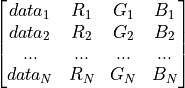
datarange (list) – (1, 2) Minimum and Maximum of plotted datarange [MIN, MAX] (default: automatic).
domain_IDs (int or list of int) – Domain IDs surface plot: Index of surface where the data is plotted on (Default: 0) volume plot: Specify the domains IDs to show in plot (default: all) Attention! Has to be included in the dataset under the name ‘tissue’! e.g. for SimNIBS:
- 1 -> white matter (WM)
- 2 -> grey matter (GM)
- 3 -> cerebrospinal fluid (CSF)
- 4 -> skull
- 5 -> skin
domain_label (str) – Label of the dataset which contains the domain IDs (default: ‘tissue_type’).
edges (BOOL) – Show edges of mesh.
fname_in (str or list of str) – Filenames of input files, 2 possibilities:
- .xdmf-file: filename of .xmdf (needs the corresponding .hdf5 file(s) in the same folder)
- .hdf5-file(s): filename(s) of .hdf5 file(s) containing the data and the geometry. The data can be provided in the first hdf5 file and the geometry can be provided in the second file. However, both can be also provided in a single hdf5 file.
fname_png (str) – Name of output .png file (incl. path).
fname_vtu_volume (str) – Name of .vtu volume file containing volume data (incl. path).
fname_vtu_surface (str) – Name of .vtu surface file containing surface data (incl. path) (to distinguish tissues).
fname_vtu_coil (str) – Name of coil .vtu file (incl. path) (optional).
info (str) – Information about the plot the settings are belonging to.
interpolate (bool) – Interpolate data for visual smoothness.
NanColor (list of float) –
1. RGB color values for “Not a Number” values (range 0 … 1).
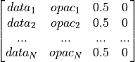
opacitymap (np.ndarray) – Points defining the piecewise linear opacity transfer function (transparency) (default: no transparency) connecting data values with opacity (alpha) values ranging from 0 (max. transparency) to 1 (no transparency).

$\begin{bmatrix} data_{1} & opac_1 & 0.5 & 0 \\ data_{2} & opac_2 & 0.5 & 0 \\ ... & ... & ... & ...\\ data_{N} & opac_N & 0.5 & 0 \\ \end{bmatrix}$
plot_function (str) – Function the plot is generated with:
- ’surface_vector_plot’
- ’surface_vector_plot_vtu’
- ’volume_plot’
- ’volume_plot_vtu’
png_resolution (float) – Resolution parameter of output image (1…5)
quantity (str) – Label of magnitude dataset to plot
surface_color (nparray [1 x 3]) – Color of brain surface in RGB (0…1) for better visability of tissue borders
surface_smoothing (bool) – Smooth the plotted surface (True/False)
show_coil (bool, default: True) – show coil if present in dataset as block termed ‘coil’
vcolor (nparray of float [N_vecs x 3]) – Array containing the RGB values between 0…1 of the vector groups in dataset to plot
vector_mode (dict) – dict key determines the type how many vectors are shown:
- ’All Points’
- ’Every Nth Point’
- ’Uniform Spatial Distribution’
dict value (int) is the corresponding number of vectors
- ’All Points’ (not set)
- ’Every Nth Point’ (every Nth vector is shown in the grid)
- ’Uniform Spatial Distribution’ (not set)
view (list) – Camera position and angle [[3 x CameraPosition], [3 x CameraFocalPoint], [3 x CameraViewUp], 1 x CameraParallelScale]
viewsize (nparray [1 x 2]) – Set size of exported image in pixel [width x height] will be extra scaled by parameter png_resolution
vlabels (list of str) – Labels of vector datasets to plot (other present datasets are ignored)
vscales (list of float) – Scale parameters of vector groups to plot
vscale_mode (list of str [N_vecs x 1]) – List containing the type of vector scaling:
- ’off’: all vectors are normalized
- ’vector’: vectors are scaled according to their magnitudeeee

pynibs.para.crop_data_hdf5_to_datarange(ps)¶

Crops the data (quantity) in .hdf5 data file to datarange and overwrites the original .hdf5 data file pointed by the .xdmf file.

Parameters:

ps (dict) – Plot settings dictionary created with create_plotsettings_dict(plot_function)

Returns:

fn_hdf5 (str) – Filename (incl. path) of data .hdf5 file (read from .xmdf file)
<File> (.hdf5 file) – *_backup.hdf5 backup file of original .hdf5 data file
<File> .hdf5 file – Cropped data

pynibs.para.crop_image(fname_image, fname_image_cropped)¶

Remove surrounding empty space around an image. This implemenation assumes that the surrounding space has the same colour as the top leftmost pixel.

Parameters:: fname_image (str) – Filename of image to be cropped
Returns:: <File> – Cropped image file saved as “fname_image_cropped”
Return type:: .png file

pynibs.para.surface_vector_plot(ps)¶

Generate plot with Paraview from data in .hdf5 file(s).

Parameters:: ps (dict) – Plot settings dict initialized with create_plot_settings_dict(plotfunction_type=’surface_vector_plot’)
Returns:: <File> – Generated plot
Return type:: .png file

pynibs.para.surface_vector_plot_vtu(ps)¶

Generate plot with Paraview from data in .vtu file.

Parameters:: ps (dict) – Plot settings dict initialized with create_plot_settings_dict(plotfunction_type=’surface_vector_plot_vtu’)
Returns:: <File> – Generated plot
Return type:: .png file

pynibs.para.volume_plot(ps)¶

Generate plot with Paraview from data in .hdf5 file.

Parameters:: ps (dict) – Plot settings dict initialized with create_plot_settings_dict(plotfunction_type=’’volume_plot’’)
Returns:: <File> – Generated plot
Return type:: .png file

pynibs.para.volume_plot_vtu(ps)¶

Generate plot with Paraview from data in .vtu file.

Parameters:: ps (dict) – Plot settings dict initialized with create_plot_settings_dict(plotfunction_type=’’volume_plot_vtu’’)
Returns:: <File> – Generated plot
Return type:: .png file

pynibs.para.write_vtu(fname, data_labels, points, connectivity, idx_start, data)¶

Writes data in tetrahedra centers into .vtu file, which can be loaded with Paraview.

Parameters:

fname (str) – Name of .vtu file (incl. path)
data_labels (list with N_data str) – Label of each dataset
points (array of float [N_points x 3]) – Coordinates of vertices
connectivity (array of int [N_tet x 4]) – Connectivity of points forming tetrahedra
idx_start (int) – Smallest index in connectivity matrix, defines offset w.r.t Python indexing, which starts at ‘0’
*data (array(s) [N_tet x N_comp(N_data)]) – Arrays containing data in tetrahedra center multiple components per dataset possible e.g. [Ex, Ey, Ez]

Returns:

<File> – Geometry and data information

Return type:

.vtu file

pynibs.para.write_vtu_coilpos(fname_geo, fname_vtu)¶

Read dipole data of coil (position and magnitude of each dipole) from geo file and store it as vtu file.

Parameters:

fname_geo (str) – .geo file from SimNIBS.
fname_vtu (str) – .vtu output file. Nodes and nodedata.

Returns:

<File> – Magnetic dipoles of the TMS coil

Return type:

.vtu file

pynibs.para.write_vtu_mult(fname, data_labels, points, triangles, tetrahedras, idx_start, *data)¶

Writes data in triangles and tetrahedra centers into .vtu file, which can be loaded with Paraview.

Parameters:

fname (str) – Name of .vtu file (incl. path)
data_labels (list of str [N_data]) – Label of each dataset
points (nparray of float [N_points x 3]) – Coordinates of vertices
triangles (nparray of int [N_tri x 3]) – Connectivity of points forming triangles
tetrahedras (nparray of int [N_tri x 4]) – Connectivity of points forming tetrahedra idx_start: int smallest index in connectivity matrix, defines offset w.r.t python indexing, which starts at ‘0’
*data (nparray(s) [N_tet x N_comp(N_data)]) – Arrays containing data in tetrahedra center multiple components per dataset possible e.g. [Ex, Ey, Ez]

Returns:

<File> – Geometry and data information

Return type:

.vtu file

pynibs.roi module¶

class pynibs.roi.CorticalLayer(create_key, id, volumetric_mesh=None, roi=None, depth=None, path=None, surface=None)¶

Bases: object

class Settings¶

Bases: object

GRID_POINTS_PER_MM = 1.5¶

NUM_TRIANGLE_SMOOTHING_STEPS = 30¶

ROI_SIZE_OFFSET = 5¶

TAG_GRAY_MATTER_SURF = 1002¶

TAG_GRAY_MATTER_VOL = 2¶

TAG_WHITE_MATTER_SURF = 1001¶

TAG_WHITE_MATTER_VOL = 1¶

classmethod create_in_bbox(id, bbox, depth, volmesh)¶

Factory method for constructing a CorticalLayer-object within a region-of-interest and a specified cortical depth.

Parameters:

id (str) – Identifier of the layer.
bbox (List[float]) – List of bounding values around the ROI box: [x_min, x_max, y_min, y_max, z_min, z_max].
depth (float) – Normalized distance of the layer from gray matter surface. Provide values in the open interval (0,1)
volmesh (simnibs.Msh) – The tetrahedral volume mesh, in which the layer should be generated.

classmethod create_in_roi(id, roi, depth, volmesh)¶

Factory method for constructing a CorticalLayer-object within a region-of-interest and a specified cortical depth.

Parameters:

id (str) – Identifier of the layer.
roi (RegionOfInterestSurface instance) – RegionOfInterestSurface
depth (float) – Normalized distance of the layer from gray matter surface. Provide values in the open interval (0,1)
volmesh (simnibs.Msh) – The tetrahedral volume mesh, in which the layer should be generated.

static crop_mesh_with_box(mesh, roi, keep_elements=False)¶

Returns the cropped mesh with all points that are inside the region of interest

Parameters:

keep_elements (bool, default = False) – If True, keeps elements with at least one point in roi, else removes them.
mesh (simnibs.Msh) – The mesh that is supposed to be cropped.
roi (List[float]) – The bounding box of the region of interest which the mesh should be cropped to. [x-min, x-max, y-min, y-max, z-min, z-max]

Returns:

mesh_cropped – The cropped mesh.

Return type:

simnibs.Msh

static crop_mesh_with_surface(mesh, roi, keep_elements=False, radius=3)¶

Returns the cropped mesh with all points that are close to the surface of interest

Parameters:

keep_elements (bool, default = False) – If True, keeps elements with at least one point in roi, else removes them.
mesh (simnibs.Msh) – The mesh that is supposed to be cropped.
roi (RegionOfInterestSurface instance) – RegionOfInterestSurface
radius (float, default = 3) – Search radius of mesh elements around ROI nodes

Returns:

mesh_cropped – The cropped mesh.

Return type:

simnibs.Msh

generate_layer(depth, roi)¶

Create the geometry of the layer at the specified depth using marching cubes.

Parameters:

depth (float) – The depth below the GM surface at which the layer should be generated; in [0,1].
roi (RegionOfInterestSurface instance) – RegionOfInterestSurface

get_evenly_spaced_element_subset(elements_per_square_mm)¶

Subsample the surface representation of the ayer.

Parameters:: elements_per_square_mm (float) – Number of triangles per mm^2 in the layer.
Returns:: selected elements – List of indices of selected elements as a result of the subsampling.
Return type:: Typing.List[int]

get_smoothed_normals()¶

Computed the smoothed normals of the surface representation of this layer.

Note: For the later stages, we don’t want a smoothed surface, but smooth normals in order to maintain the location of the cells, but orient them more smoothly. Therefore, we use smoothed normals, e.g. for the computation of the theta angle, but do not smooth the entire layer surface.

Returns:: normals – The tetrahedral volume mesh, in which the layer should be generated.
Return type:: np.ndarray

classmethod init_from_file(id, fn)¶

Factory method for constructing a CorticalLayer-object from a file.

Parameters:

id (str) – Identifier of the layer.
fn (str) – File path to a region of interest surfe (e.g. midlayer).

classmethod init_from_surface(id, surf)¶

Factory method for constructing a CorticalLayer-object from a Simnibs-surface object.

Parameters:

id (str) – Identifier of the layer.
surf (simnibs.Msh) – The surface representation of an already existing layer (e.g. midlayer).

remove_unconnected_surfaces()¶: Remove elements small unconnected element-clusters from this layer.

static roi_bbox_from_points(points, offset=0)¶

Find the minimal bounding box around the provided points.

Parameters:

points (simnibs.Msh) – The tetrahedral volume mesh, in which the layer should be generated.
offset (float) – Normalized distance of the layer from gray matter surface. Provide values in the open interval (0,1)

Returns:

bounding_box – List of bounding values around the provided points: [x_min, x_max, y_min, y_max, z_min, z_max].

Return type:

List[float]

save(fn)¶

Save the current surface representation of this CorticalLayer instance at the specified location.

Parameters:: fn (str) – Target file name of the surface-file of this layer.

class pynibs.roi.RegionOfInterestSurface¶

Bases: object

Region of interest (surface).

node_coord_up¶

(N_points, 3) Coordinates (x,y,z) of upper surface nodes

Type:: np.ndarray

node_coord_mid¶

(N_points, 3) Coordinates (x,y,z) of middle surface nodes

Type:: np.ndarray

node_coord_low¶

(N_points, 3) Coordinates (x,y,z) of lower surface nodes

Type:: np.ndarray

node_number_list¶

(N_points, 3) Connectivity matrix of triangles

Type:: np.ndarray

delta¶

Distance parameter between WM and GM (0 -> WM, 1 -> GM)

Type:: float

tet_idx_tri_center_up¶

Tetrahedra indices of TetrahedraLinear object instance where the center points of the triangles of the upper surface are lying in

Type:: np.ndarray [N_points]

tet_idx_tri_center_mid¶

Tetrahedra indices of TetrahedraLinear object instance where the center points of the triangles of the middle surface are lying in

Type:: np.ndarray [N_points]

tet_idx_tri_center_low¶

Tetrahedra indices of TetrahedraLinear object instance where the center points of the triangles of the lower surface are lying in

Type:: np.ndarray [N_points]

tet_idx_node_coord_mid¶

(N_tri,) Tetrahedra indices of TetrahedraLinear object instance where the nodes of the middle surface are lying in

Type:: np.ndarray

tri_center_coord_up¶

(N_tri, 3) Coordinates of roi triangle center of upper surface

Type:: np.ndarray

tri_center_coord_mid¶

(N_tri, 3) Coordinates of roi triangle center of middle surface

Type:: np.ndarray

tri_center_coord_low¶

(N_tri, 3) Coordinates of roi triangle center of lower surface

Type:: np.ndarray

fn_mask¶

Filename for surface mask in subject space. .mgh file or freesurfer surface file.

Type:: string

fn_mask_avg¶

Filename for .mgh mask in fsaverage space. Absolute path or relative to mesh folder.

Type:: string

fn_mask_nii¶

Filename for .nii or .nii.gz mask. Absolute path or relative to mesh folder.

Type:: string

X_ROI¶

Region of interest [Xmin, Xmax], whole X range if empty [0,0] or None (left - right)

Type:: list of float

Y_ROI¶

Region of interest [Ymin, Ymax], whole Y range if empty [0,0] or None (anterior - posterior)

Type:: list of float

Z_ROI¶

Region of interest [Zmin, Zmax], whole Z range if empty [0,0] or None (inferior - superior)

Type:: list of float

template¶

‘MNI’, ‘fsaverage’, ‘subject’

Type:: str

center¶

Center coordinates for spherical ROI in self.template space

Type:: list of float

radius¶

Radius in [mm] for spherical ROI

Type:: float

gm_surf_fname¶

Filename(s) of GM surface generated by freesurfer (lh and/or rh) (e.g. in mri2msh: …/fs_ID/surf/lh.pial)

Type:: str or list of str

wm_surf_fname¶

Filename(s) of WM surface generated by freesurfer (lh and/or rh) (e.g. in mri2msh: …/fs_ID/surf/lh.white)

Type:: str or list of str

layer¶

Define the number of layers:

1: one layer
3: additionally upper and lower layers are generated around the central midlayer

Type:: int

decimate(fraction=0.075)¶

Subsample ROI surface based on a decimation factor and return element indices. (no Freesurfer surfaces associated with the ROI surface required)

Parameters:: fraction (float, default: .075) – Multiplied by the total number of ROI elements determines (approximately) the number of remaining ROI elements after decimation.
Returns:: ele_idx – [approx. fraction * n_ele] Element indices of the subsampled surface; sorted.
Return type:: np.ndarray of float

determine_element_idx_in_mesh(msh)¶

Determines tetrahedra indices of msh where the triangle center points of upper, middle and lower surface and the nodes of middle surface are lying in.

Parameters:

msh (pynibs.mesh.mesh_struct.TetrahedraLinear) – TetrahedraLinear object.

Returns:

RegionOfInterestSurface.tet_idx_tri_center_up (np.ndarray) – (N_points) Tetrahedra indices of TetrahedraLinear object instance where the center points of the triangles of the upper surface are lying in.
RegionOfInterestSurface.tet_idx_tri_center_mid (np.ndarray) – (N_points) Tetrahedra indices of TetrahedraLinear object instance where the center points of the triangles of the middle surface are lying in.
RegionOfInterestSurface.tet_idx_tri_center_low (np.ndarray) – (N_points) Tetrahedra indices of TetrahedraLinear object instance where the center points of the triangles of the lower surface are lying in.
RegionOfInterestSurface.tet_idx_node_coord_mid (np.ndarray) – (N_tri) Tetrahedra indices of TetrahedraLinear object instance where the nodes of the middle surface are lying in.

generate_cortical_laminae(head_model_mesh, bbox=None, laminae=(0.06, 0.4, 0.55, 0.65, 0.85), layer_ids=('L1', 'L23', 'L4', 'L5', 'L6'))¶

Create the cortical layering with the provided laminar depths.

Defaults to the standard depths of the laminae in the neo-cortex from layer I to VI from “Simulation of transcranial magnetic stimulation in head model with morphologically-realistic cortical neurons”, Aberra et al., https://doi.org/10.1016/j.brs.2019.10.002

Parameters:

head_model_mesh (simnibs.Msh) – The head model volume mesh. Inside the GM compartment of this mesh, the layering will be generated.
bbox (np.ndarray, optional) – Bounding coordinates of the region of interest. Optional, if the mid-layer surface is already existing (and can thus be used to determine the bounding coordinates).
laminae (Dict[str,float] | Tuple) – List of depths of the individual to-be created lamiae.

make_GM_WM_surface(gm_surf_fname=None, wm_surf_fname=None, midlayer_surf_fname=None, mesh_folder=None, delta=0.5, x_roi=None, y_roi=None, z_roi=None, layer=1, fn_mask=None, refine=False)¶

Generating a surface between WM and GM in a distance of delta 0…1 for ROI, given by Freesurfer mask or coordinates.

Parameters:

gm_surf_fname (str or list of str) – Filename(s) of GM FreeSurfer surface(s) (lh and/or rh). Either relative to mesh_folder (fs_ID/surf/lh.pial) or absolute (/full/path/to/lh.pial)
wm_surf_fname (str or list of str) – Filename(s) of WM FreeSurfer surface(s) (lh and/or rh) Either relative to mesh_folder (fs_ID/surf/lh.white) or absolute (/full/path/to/lh.white)
midlayer_surf_fname (str or list of str) – Filename(s) of midlayer surface (lh and/or rh) Either relative to mesh_folder (fs_ID/surf/lh.central) or absolute (/full/path/to/lh.central)
mesh_folder (str) – Root folder of mesh, Needed if paths above are given relative, or refine=True
m2m_mat_fname ([defunct]) – Filename of mri2msh transformation matrix (e.g. in mri2msh: …/m2m_ProbandID/MNI2conform_6DOF.mat)
delta (float) –
Distance parameter where surface is generated 0…1 (default: 0.5)
- 0 -> WM surface
- 1 -> GM surface
x_roi (list of float) – Region of interest [Xmin, Xmax], whole X range if empty [0,0] or None (left - right)
y_roi (list of float) – Region of interest [Ymin, Ymax], whole Y range if empty [0,0] or None (anterior - posterior)
z_roi (list of float) – Region of interest [Zmin, Zmax], whole Z range if empty [0,0] or None (inferior - superior)
layer (int) –
Define the number of layers:
- 1: one layer
- 3: additionally upper and lower layers are generated around the central midlayer
fn_mask (str) – Filename for FreeSurfer .mgh mask.
refine (bool, optional, default: False) – Refine ROI by splitting elements

Returns:

node_coord_up (np.ndarray of float [N_roi_points x 3]) – Node coordinates (x, y, z) of upper epsilon layer of ROI surface
node_coord_mid (np.ndarray of float [N_roi_points x 3]) – Node coordinates (x, y, z) of ROI surface
node_coord_low (np.ndarray of float [N_roi_points x 3]) – Node coordinates (x, y, z) of lower epsilon layer of ROI surface
node_number_list (np.ndarray of int [N_roi_tri x 3]) – Connectivity matrix of intermediate surface layer triangles
delta (float) – Distance parameter where surface is generated 0…1 (default: 0.5)
- 0 -> WM surface
- 1 -> GM surface
tri_center_coord_up (np.ndarray of float [N_roi_tri x 3]) – Coordinates (x, y, z) of triangle center of upper epsilon layer of ROI surface
tri_center_coord_mid (np.ndarray of float [N_roi_tri x 3]) – Coordinates (x, y, z) of triangle center of ROI surface
tri_center_coord_low (np.ndarray of float [N_roi_tri x 3]) – Coordinates (x, y, z) of triangle center of lower epsilon layer of ROI surface
fn_mask (str) – Filename for freesurfer mask. If given, this is used instead of *_ROIs
X_ROI (list of float) – Region of interest [Xmin, Xmax], whole X range if empty [0,0] or None (left - right)
Y_ROI (list of float) – Region of interest [Ymin, Ymax], whole Y range if empty [0,0] or None (anterior - posterior)
Z_ROI (list of float) – Region of interest [Zmin, Zmax], whole Z range if empty [0,0] or None (inferior - superior)

Example

make_GM_WM_surface(self, gm_surf_fname, wm_surf_fname, delta, X_ROI, Y_ROI, Z_ROI)
make_GM_WM_surface(self, gm_surf_fname, wm_surf_fname, delta, mask_fn, layer=3)

project_on_midlayer(target, verbose=False)¶

Project a coordinate on the nearest midlayer node

Parameters:

target (np.ndarray) – Coordinate to project as (3,) array
verbose (bool) – Print some verbosity information. Default: False

Returns:

target_proj – Node coordinate of nearest midlayer node.

Return type:

np.ndarray

subsample(dist=10, fn_sphere=None)¶

Subsample ROI surface based on a spacing and return element indices (Freesurfer surfaces associatd with the ROI surface required)

Parameters:

dist (float) – Distance in mm the subsampled points lie apart.
fn_sphere (str) – Name of ?.sphere file (freesurfer).

Returns:

ele_idx – (n_ele) Element indices of the subsampled surface.

Return type:

ndarray of float

class pynibs.roi.RegionOfInterestVolume¶

Bases: object

Region of interest (volume) class

node_coord¶

Coordinates (x,y,z) of ROI tetrahedra nodes.

Type:: np.ndarray [N_points x 3]

tet_node_number_list¶

Connectivity matrix of ROI tetrahedra.

Type:: np.ndarray [N_tet_roi x 3]

tri_node_number_list¶

Connectivity matrix of ROI tetrahedra.

Type:: np.ndarray [N_tri_roi x 3]

tet_idx_node_coord¶

Tetrahedra indices of TetrahedraLinear object instance where the ROI nodes are lying in.

Type:: np.ndarray [N_points]

tet_idx_tetrahedra_center¶

(N_tet_roi) Tetrahedra indices of TetrahedraLinear object instance where the center points of the ROI tetrahedra are lying in.

Type:: np.ndarray

tet_idx_triangle_center¶

(N_tri_roi) Tetrahedra indices of TetrahedraLinear object instance where the center points of the ROI triangle are lying in. If the ROI is directly generated from the msh instance using “make_roi_volume_from_msh”, these indices are the triangle indices of the head mesh since the ROI mesh and the head mesh are overlapping. If the ROI mesh is not the same as the head mesh, the triangle center of the ROI mesh are always lying in a tetrahedra of the head mesh (these indices are given in this case).

Type:: np.ndarray

make_roi_volume_from_msh(msh, volume_type='box', x_roi=None, y_roi=None, z_roi=None)¶

Generate region of interest (volume) and extract nodes, triangles and tetrahedra from msh instance.

Parameters:

msh (pynibs.mesh.mesh_struct.TetrahedraLinear) – Mesh object instance of type TetrahedraLinear
volume_type (str) – Type of ROI (‘box’ or ‘sphere’)
x_roi (list of float) –
- type = ‘box’: [Xmin, Xmax] (in mm), whole X range if empty [0,0] or None (left - right)
- type = ‘sphere’: origin [x,y,z]
y_roi (list of float) –
- type = ‘box’: [Ymin, Ymax] (in mm), whole Y range if empty [0,0] or None (anterior - posterior)
- type = ‘sphere’: radius (in mm)
z_roi (list of float) –
- type = ‘box’: [Zmin, Zmax] (in mm), whole Z range if empty [0,0] or None (inferior - superior)
- type = ‘sphere’: None

Returns:

RegionOfInterestVolume.node_coord (np.ndarray [N_points x 3]) – Coordinates (x,y,z) of ROI tetrahedra nodes
RegionOfInterestVolume.tet_node_number_list (np.ndarray [N_tet_roi x 3]) – Connectivity matrix of ROI tetrahedra
RegionOfInterestVolume.tri_node_number_list (np.ndarray [N_tri_roi x 3]) – Connectivity matrix of ROI tetrahedra
RegionOfInterestVolume.tet_idx_node_coord (np.ndarray [N_points]) – Tetrahedra indices of TetrahedraLinear object instance where the ROI nodes are lying in
RegionOfInterestVolume.tet_idx_tetrahedra_center (np.ndarray [N_tet_roi]) – Tetrahedra indices of TetrahedraLinear object instance where the center points of the ROI tetrahedra are lying in
RegionOfInterestVolume.tet_idx_triangle_center (np.ndarray [N_tri_roi]) – Tetrahedra indices of TetrahedraLinear object instance where the center points of the ROI triangle are lying in. If the ROI is directly generated from the msh instance using “make_roi_volume_from_msh”, these indices are the triangle indices of the head mesh since the ROI mesh and the head mesh are overlapping. If the ROI mesh is not the same as the head mesh, the triangle center of the ROI mesh are always lying in a tetrahedra of the head mesh (these indices are given in this case)

pynibs.roi.clean_roi(img, vox_thres=0.5, fn_out=None)¶

Remove values < vox thres from image.

Parameters:

img (str or nibabel.nifti1.Nifti1Image) –
vox_thres (float, optional) –
fn_out (str) –

Returns:

img_thres (nibabel.nifti1.Nifti1Image)
img_thres (<file>) – If fn_out is specified, thresholded image is saved here

pynibs.roi.create_refine_spherical_roi(center, radius, final_tissues_nii, out_fn, target_size=0.5, outside_size=None, outside_factor=3, out_spher_fn=None, tissue_types=None, verbose=False)¶

Create a spherical roi nifti for simnibs 4 refinement. Only tissue types accoring to _tissue_types will be refined.

Use the resulting output file as input for –sizing_field in SimNIBS-4/simnibs/cli/meshmesh.py

Parameters:

center (list of float) – Center of spherical ROI in mm
radius (float) – Radius of spherical ROI in mm
final_tissues_nii (string or nib.nifti1.Nifti1Image) – final_tissues.nii.gz to create roi for.
out_fn (str) – Final output filename
target_size (float, default = 0.5) – Target element size of refined areas in mm (?)
outside_size (float, default = None) – Element size outside of target size.
outside_factor (float, default = None) – Distance factor to define the ‘outside’ area: oudsidefactor * radius -> outside
out_spher_fn (str, optional) – Output filename of orignal, raw spherical ROI
tissue_types (list of float, default = [1,2,3]) – Which tissue types to refine. Defaults to WM, GM, CSF
verbose (bool, optional, default=False) – Print additional information

pynibs.roi.determine_element_idx_in_mesh(fname, msh, points, compute_baricentric=False)¶

Finds the tetrahedron that contains each of the described points using a stochastic walk algorithm. Implemented from Devillers et al. (2002) [1]

Parameters:

msh (pynibs.mesh.mesh_struct.TetrahedraLinear) –
fname (str or None) – Filename of saved .txt file containing the element indices (no data is saved when fname=None or fname=’’)
points (np.ndarray (N, 3) or list of np.ndarray) – List of points to be queried
compute_baricentric (bool) – Wether or not to compute baricentric coordinates of the points

Returns:

th_with_points (np.ndarray) – List with the tetrahedron that contains each point. If the point is outside the mesh, the value will be -1
baricentric (np.ndarray [n, 4](if compute_baricentric == True)) – Baricentric coordinates of point. If the point is outside, a list of zeros

Notes

[1]

Devillers, Olivier, Sylvain Pion, and Monique Teillaud. “Walking in a triangulation.” International Journal of Foundations of Computer Science 13.02 (2002): 181-199.

pynibs.roi.elem_workhorse(chunk, points_out, P1_all, P2_all, P3_all, P4_all, N_points_total, N_CPU)¶

Parameters:

chunk (np.ndarray) – Indices of points the CPU thread is computing the element indices for
points_out (np.ndarray of float) – (N_points, 3) Coordinates of points, the tetrahedra indices are computed for
P1_all (np.ndarray of float) –
(N_tet –
tetrahedra (3) Coordinates of first point of) –
P2_all (np.ndarray of float) – (N_tet, 3) Coordinates of second point of tetrahedra
P3_all (np.ndarray of float) – (N_tet, 3) Coordinates of third point of tetrahedra
P4_all (np.ndarray of float) – (N_tet, 3) Coordinates of fourth point of tetrahedra
N_points_total (int) – Total number of points
N_CPU (int) – Number of CPU cores to use

Returns:

tet_idx_local

Return type:

np.ndarray of int (N_points,)

pynibs.roi.get_mask(areas, fn_annot, fn_inflated_fs, fn_out)¶

Determine freesurfer average mask .overlay file, which is needed to generate subject specific ROIs.

Parameters:

areas (list of str) – Brodmann areas (e.g. [‘Brodmann.6’, ‘Brodmann.4’, ‘Brodmann.3’, ‘Brodmann.1’])
fn_annot (str) – Annotation file of freesurfer (e.g. ‘FREESURFER_DIR/fsaverage/label/lh.PALS_B12_Brodmann.annot’)
fn_inflated_fs (str) – Inflated surface of freesurfer average (e.g. ‘FREESURFER_DIR/fsaverage/surf/lh.inflated’)
fn_out (str) – Filename of .overlay file of freesurfer mask

Returns:

<File> – fn_out.overlay file of freesurfer mask

Return type:

.overlay file

pynibs.roi.get_sphere_in_nii(center, radius, nii=None, out_fn=None, thresh_by_nii=True, val_in=1, val_out=0, outside_val=0, outside_radius=inf)¶

Computes a spherical ROI for a given Nifti image (defaults to SimNIBS MNI T1 tissue). The ROI area is defined in nifti coordinates. By default, everything inside the ROI is set to 1, areas outside = 0. The ROI is further thresholded by the nifti. A nib.Nifti image is returned and optionally saved.

Parameters:

center (array-like) – X, Y, Z coordinates in nifti space
radius (float) – radius of sphere
nii (string or nib.nifti1.Nifti1Image, optional) – The nifti image to work with.
out_fn (string, optional) – If provided, sphere ROI image is saved here
outside_val (float, default = None) – Value outside of outside_radius.
outside_radius (float, default = None) – Distance factor to define the ‘outside’ area: oudsidefactor * radius -> outside
thresh_by_nii (bool, optional) – Mask sphere by nii != 0
val_in (float, optional) – Value within ROI
val_out (float, optional) – Value outside ROI

Returns:

sphere_img (nib.nifti1.Nifti1Image)
sphere_img (<file>, optional)

Raises:

ValueError – If the final ROI is empty.

pynibs.roi.load_roi_surface_obj_from_hdf5(fname)¶

Loading and initializing RegionOfInterestSurface object/s from .hdf5 mesh file.

Parameters:: fname (str) – Filename (incl. path) of .hdf5 mesh file, e.g. from subject.fn_mesh_hdf5
Returns:: RegionOfInterestSurface – RegionOfInterestSurface
Return type:: pynibs.roi.RegionOfInterestSurface or list of pynibs.roi.RegionOfInterestSurface

pynibs.roi.make_GM_WM_surface(gm_surf_fname, wm_surf_fname, mesh_folder, midlayer_surf_fname=None, delta=0.5, x_roi=None, y_roi=None, z_roi=None, layer=1, fn_mask=None, refine=False)¶

Generating a surface between WM and GM in a distance of delta 0…1 for ROI, given by freesurfer mask or coordinates.

Parameters:

gm_surf_fname (str or list of str) – Filename(s) of GM surface generated by freesurfer (lh and/or rh) (e.g. in mri2msh: fs_ID/surf/lh.pial)
wm_surf_fname (str or list of str) – Filename(s) of WM surface generated by freesurfer (lh and/or rh) (e.g. in mri2msh: fs_ID/surf/lh.white)
mesh_folder (str) – Path of mesh (parent directory)
midlayer_surf_fname (str or list of str) – filename(s) of midlayer surface generated by headreco (lh and/or rh) (e.g. in headreco: fs_ID/surf/lh.central) (after conversion)
m2m_mat_fname ([defunct]) – Filename of mri2msh transformation matrix (e.g. in mri2msh: m2m_ProbandID/MNI2conform_6DOF.mat)
delta (float) –
Distance parameter where surface is generated 0…1 (default: 0.5)
- 0 -> WM surface
- 1 -> GM surface
x_roi (list of float or None) – Region of interest [Xmin, Xmax], whole X range if empty [0,0] or None (left - right)
y_roi (list of float or None) – Region of interest [Ymin, Ymax], whole Y range if empty [0,0] or None (anterior - posterior)
z_roi (list of float or None) – Region of interest [Zmin, Zmax], whole Z range if empty [0,0] or None (inferior - superior)
layer (int) –
Define the number of layers:
- 1: one layer
- 3: additionally upper and lower layers are generated around the central midlayer
fn_mask (string or None) – Filename for freesurfer mask. If given, this is used instead of *_ROIs
refine (bool, optional, default: False) – Refine ROI by splitting elements

Returns:

if layer == 3
surface_points_upper (np.ndarray of float) – (N_points, 3) Coordinates (x, y, z) of surface + epsilon (in GM surface direction)
surface_points_middle (np.ndarray of float) – (N_points, 3) Coordinates (x, y, z) of surface
surface_points_lower (np.ndarray of float) – (N_points, 3) Coordinates (x, y, z) of surface - epsilon (in WM surface direction)
connectivity (np.ndarray of int) – (N_tri x 3) Connectivity of triangles (indexation starts at 0!)
else
surface_points_middle (np.ndarray of float) – (N_points, 3) Coordinates (x, y, z) of surface
connectivity (np.ndarray of int) – (N_tri x 3) Connectivity of triangles (indexation starts at 0!)

Example

make_GM_WM_surface(self, gm_surf_fname, wm_surf_fname, delta, X_ROI, Y_ROI, Z_ROI)
make_GM_WM_surface(self, gm_surf_fname, wm_surf_fname, delta, mask_fn, layer=3)

pynibs.roi.nii2msh(mesh, m2m_dir, nii, out_folder, hem, out_fsaverage=False, roi_name='ROI')¶

Transform a nifti ROI image to subject space .mgh file.

Parameters:

mesh (simnibs.Mesh or str) –
m2m_dir (str) –
nii (nibabel.nifti1.Nifti1Image or str) –
out_folder (str) –
hem (str) – ‘lh’ or ‘rh’
out_fsaverage (bool) –
roi_name (str) – How to name the ROI

Returns:

roi – f”{out_folder}/{hem}.mesh.central.{roi_name}”

Return type:

file

pynibs.subject module¶

class pynibs.subject.Subject(subject_id, subject_folder)¶

Bases: object

Subject containing subject specific information, like mesh, roi, uncertainties, plot settings.

self.id¶

Subject id from MPI database

Type:: str

Notes

Initialization

Parameters

idstr: Subject id
fn_meshstr: .msh or .hdf5 file containing the mesh information

Subject.seg, segmentation information dictionary

fn_lh_wmstr: Filename of left hemisphere white matter surface
fn_rh_wmstr: Filename of right hemisphere white matter surface
fn_lh_gmstr: Filename of left hemisphere grey matter surface
fn_rh_gmstr: Filename of right hemisphere grey matter surface
fn_lh_curvstr: Filename of left hemisphere curvature data on grey matter surface
fn_rh_curvstr: Filename of right hemisphere curvature data on grey matter surface

Subject.mri, mri information dictionary

fn_mri_T1str: Filename of T1 image
fn_mri_T2str: Filename of T2 image
fn_mri_DTIstr: Filename of DTI dataset
fn_mri_DTI_bvecstr: Filename of DTI bvec file
fn_mri_DTI_bvalstr: Filename of DTI bval file
fn_mri_conformstr: Filename of conform T1 image resulting from SimNIBS mri2mesh function

Subject.ps, plot settings dictionary

see plot functions in para.py for more details

Subject.exp, experiment dictionary

infostr: General information about the experiment
datestr: Date of experiment (e.g. 01/01/2018)
fn_tms_navstr: Path to TMS navigator folder
fn_datastr: Path to data folder or files
fn_exp_csvstr: Filename of experimental data .csv file containing the merged experimental data information
fn_coilstr: Filename of .ccd or .nii file of coil used in the experiment (contains ID)
fn_mri_niistr: Filename of MRI .nii file used during the experiment
condstr or list of str: Conditions in the experiment in the recorded order (e.g. [‘PA-45’, ‘PP-00’])
experimenterstr: Name of experimenter who conducted the experiment
incidentsstr: Description of special events occured during the experiment

Subject.mesh, mesh dictionary

infostr: Information about the mesh (e.g. dicretization etc)
fn_mesh_mshstr: Filename of the .msh file containing the FEM mesh
fn_mesh_hdf5str: Filename of the .hdf5 file containing the FEM mesh
seg_idxint: Index indicating to which segmentation dictionary the mesh belongs

Subject.roi region of interest dictionary

typestr: Specify type of ROI (‘surface’, ‘volume’)
infostr: Info about the region of interest, e.g. “M1 midlayer from freesurfer mask xyz”
regionlist of str or float: Filename for freesurfer mask or [[X_min, X_max], [Y_min, Y_max], [Z_min, Z_max]]
deltafloat: Distance parameter between WM and GM (0 -> WM, 1 -> GM) (for surfaces only)

add_experiment_info(exp_dict)¶

Adding information about a particular experiment.

Parameters:: exp_dict (dict of dict or list of dict) – Dictionary containing information about the experiment

Notes

Adds Attributes

explist of dict: Dictionary containing information about the experiment

add_mesh_info(mesh_dict)¶

Adding filename information of the mesh to the subject object (multiple filenames possible).

Parameters:: mesh_dict (dict or list of dict) – Dictionary containing the mesh information

Notes

Adds Attributes

Subject.meshlist of dict: Dictionaries containing the mesh information

add_mri_info(mri_dict)¶

Adding MRI information to the subject object (multiple MRIs possible).

Parameters:: mri_dict (dict or list of dict) – Dictionary containing the MRI information of the subject

Notes

Adds Attributes

Subject.mrilist of dict: Dictionary containing the MRI information of the subject

add_plotsettings(ps_dict)¶

Adding ROI information to the subject object (multiple ROIs possible).

Parameters:: ps_dict (dict or list of dict) – Dictionary containing plot settings of the subject

Notes

Adds Attributes

Subject.pslist of dict: Dictionary containing plot settings of the subject

add_roi_info(roi_dict)¶

Adding ROI (surface) information of the mesh with mesh_index to the subject object (multiple ROIs possible).

Parameters:: roi_dict (dict of dict or list of dict) – Dictionary containing the ROI information of the mesh with mesh_index [mesh_idx][roi_idx]

Notes

Adds Attributes

Subject.mesh[mesh_index].roilist of dict: Dictionaries containing ROI information

pynibs.subject.check_file_and_format(fname)¶

Checking existence of file and transforming to list if necessary.

Parameters:: fname (str or list of str) – Filename(s) to check
Returns:: fname – Checked filename(s) as list
Return type:: list of str

pynibs.subject.fill_from_dict(obj, d)¶

Set all attributes from d in obj.

Parameters:

obj (pynibs.Mesh or pynibs.ROI) –
d (dict) –

Returns:

obj

Return type:

pynibs.Mesh or pynibs.ROI

pynibs.subject.load_subject(fname, filetype=None)¶

Wrapper for pkl and hdf5 subject loader

Parameters:

fname (str) – endwith(‘.pkl’) | endswith(‘.hdf5’)
filetype (str) – Explicitely set file version.

Returns:

subject

Return type:

pynibs.subject.Subject

pynibs.subject.load_subject_hdf5(fname)¶

Loading subject information from .hdf5 file and returning subject object.

Parameters:: fname (str) – Filename with .hdf5 extension (incl. path)
Returns:: subject – Loaded Subject object
Return type:: pynibs.subject.Subject

pynibs.subject.load_subject_pkl(fname)¶

Loading subject object from .pkl file.

Parameters:: fname (str) – Filename with .pkl extension
Returns:: subject – Loaded Subject object
Return type:: pynibs.subject.Subject

pynibs.subject.save_subject(subject_id, subject_folder, fname, mri_dict=None, mesh_dict=None, roi_dict=None, exp_dict=None, ps_dict=None, **kwargs)¶

Saves subject information in .pkl or .hdf5 format (preferred)

Parameters:

subject_id (str) – ID of subject
subject_folder (str) – Subject folder
fname (str) – Filename with .hdf5 or .pkl extension (incl. path)
mri_dict (list of dict, optional, default: None) – MRI info
mesh_dict (list of dict, optional, default: None) – Mesh info
roi_dict (list of list of dict, optional, default: None) – Mesh info
exp_dict (list of dict, optional, default: None) – Experiment info
ps_dict (list of dict, optional, default:None) – Plot-settings info
kwargs (str or np.array) – Additional information saved in the parent folder of the .hdf5 file

Returns:

<File> – Subject information

Return type:

.hdf5 file

pynibs.subject.save_subject_hdf5(subject_id, subject_folder, fname, mri_dict=None, mesh_dict=None, roi_dict=None, exp_dict=None, ps_dict=None, overwrite=True, check_file_exist=False, verbose=False, **kwargs)¶

Saving subject information in hdf5 file.

Parameters:

subject_id (str) – ID of subject
subject_folder (str) – Subject folder
fname (str) – Filename with .hdf5 extension (incl. path)
mri_dict (list of dict, optional, default: None) – MRI info
mesh_dict (list of dict, optional, default: None) – Mesh info
roi_dict (list of list of dict, optional, default: None) – Mesh info
exp_dict (list of dict or dict of dict, optional, default: None) – Experiment info
ps_dict (list of dict, optional, default:None) – Plot-settings info
overwrite (bool) – Overwrites existing .hdf5 file
check_file_exist (bool) – Hide warnings.
verbose (bool) – Print information about meshes and ROIs.
kwargs (str or np.ndarray) – Additional information saved in the parent folder of the .hdf5 file

Returns:

<File> – Subject information

Return type:

.hdf5 file

pynibs.subject.save_subject_pkl(sobj, fname)¶

Saving subject object as pickle file.

Parameters:

sobj (object) – Subject object to save
fname (str) – Filename with .pkl extension

Returns:

<File> – Subject object instance

Return type:

.pkl file

pynibs.tensor_scaling module¶

pynibs.tensor_scaling.ellipse_eccentricity(a, b)¶

Calculates the eccentricity of an 2D ellipse with the semi axis a and b. An eccentricity of 0 corresponds to a sphere and an eccentricity of 1 means complete eccentric (line) with full restriction to the other axis

Parameters:

a (float) – First semi axis parameter
b (float) – Second semi axis parameter

Returns:

e – Eccentricity (0…1)

Return type:

float

pynibs.tensor_scaling.rescale_lambda_centerized(D, s, tsc=False)¶

Rescales the eigenvalues of the matrix D according to their eccentricity. The scale factor is between 0…1 a scale factor of 0.5 would not alter the eigenvalues of the matrix D. A scale factor of 0 would unify all eigenvalues to one value such that it corresponds to a isotropic sphere. A scale factor of 1 alters the eigenvalues in such a way that the resulting ellipsoid is fully eccentric and anisotropic.

Parameters:

D (nparray of float) – (3, 3) Diffusion tensor.
s (float) – Scale parameter [0 (iso) … 0.5 (unaltered)… 1 (aniso)].
tsc (bool) – Tensor singularity correction.

Returns:

Ds – (3, 3) Scaled diffusion tensor.

Return type:

np.ndarray of float

pynibs.tensor_scaling.rescale_lambda_centerized_workhorse(D, s, tsc=False)¶

Parameters:

D (ndarray of float) – (n, 9) Diffusion tensor.
s (float) – Scale parameter [0 (iso) … 0.5 (unaltered)… 1 (aniso)].
tsc (bool) – Tensor singularity correction.

Returns:

Ds – (3, 3) Scaled diffusion tensor

Return type:

list of nparray of float

pynibs.tms_pulse module¶

pynibs.tms_pulse.biphasic_pulse(t, R=0.0338, L=1.55e-05, C=0.0001936, alpha=1089.8, f=2900)¶

Returns normalized single biphasic pulse waveform of electric field (first derivative of coil current)

Parameters:

t (ndarray of float [n_t]) – Time array in seconds
R (float, optional, default: 0.0338 Ohm) – Resistance of coil in (Ohm)
L (float, optional, default: 15.5*1e-6 H) – Inductance of coil in (H)
C (float, optional, default: 193.6*1e-6) – Capacitance of coil in (F)
alpha (float, optional, default: 1089.8 1/s) – Damping coefficient in (1/s)
f (float, optional, default: 2900 Hz) – Frequency in (Hz)

Returns:

e – Normalized electric field time course (can be scaled with electric field)

Return type:

ndarray of float [n_t]

pynibs package

pynibs package¶

Subpackages¶

Submodules¶

pynibs.coil module¶

pynibs.freesurfer module¶

pynibs.hdf5_io module¶

pynibs.muap module¶

pynibs.opt module¶

pynibs.para module¶

pynibs.roi module¶

pynibs.subject module¶

pynibs.tensor_scaling module¶

pynibs.tms_pulse module¶

Table of Contents

Previous topic

Next topic

This Page